[Sigmoid function의 문제점]
다음 단어들의 뜻을 이해해야 앞으로 이야기할 내용들이 이해될 것이다.
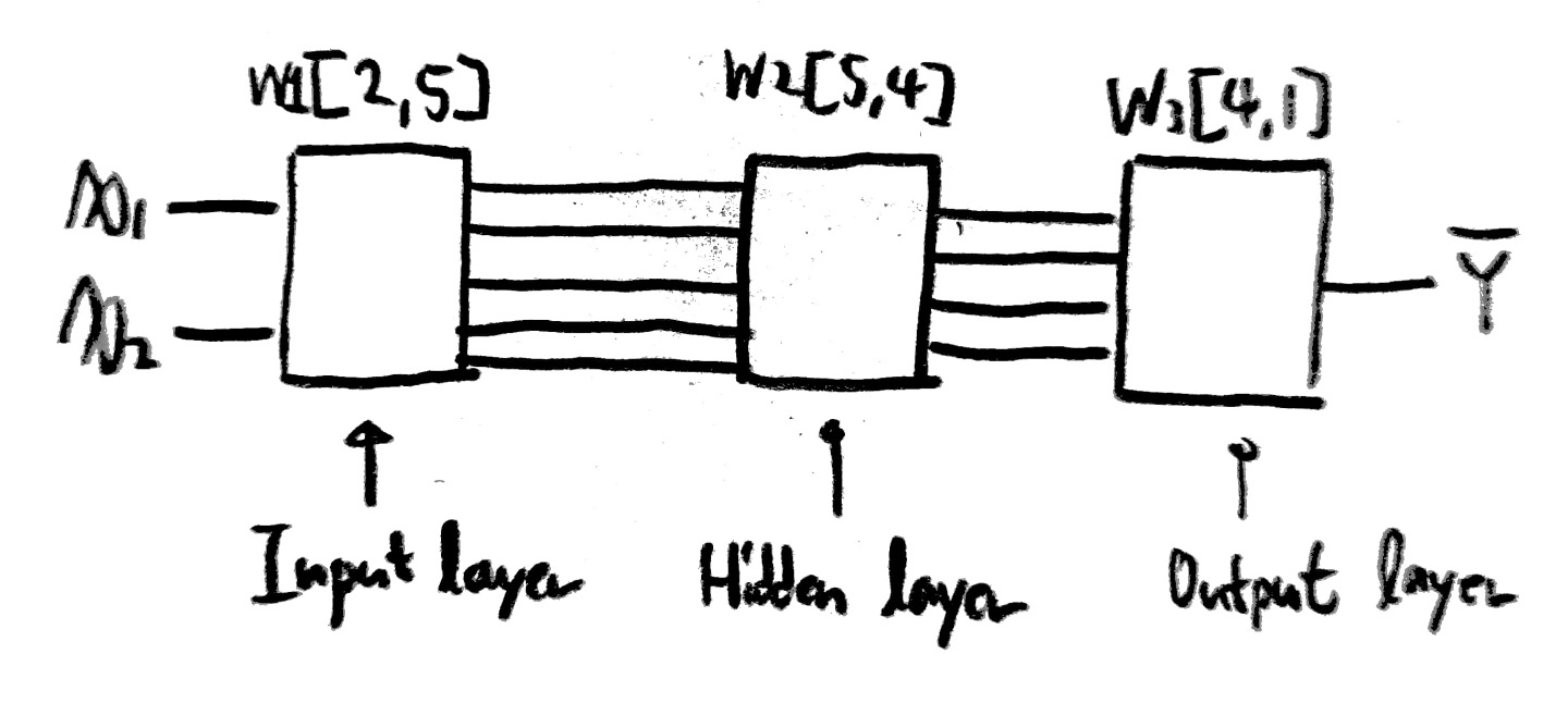
우리는 지금까지 깊은 NN을 어떻게 만드는지 넓은 NN은 어떻게 만드는지 알아보았다.
그럼 한번 XOR문제를 깊고 넓은(Deep and Wide) NN에서 사용해보라.
(대충 hidden layer가 10개 정도면 됨, sigmoid 함수를 사용해서 구현할 것)
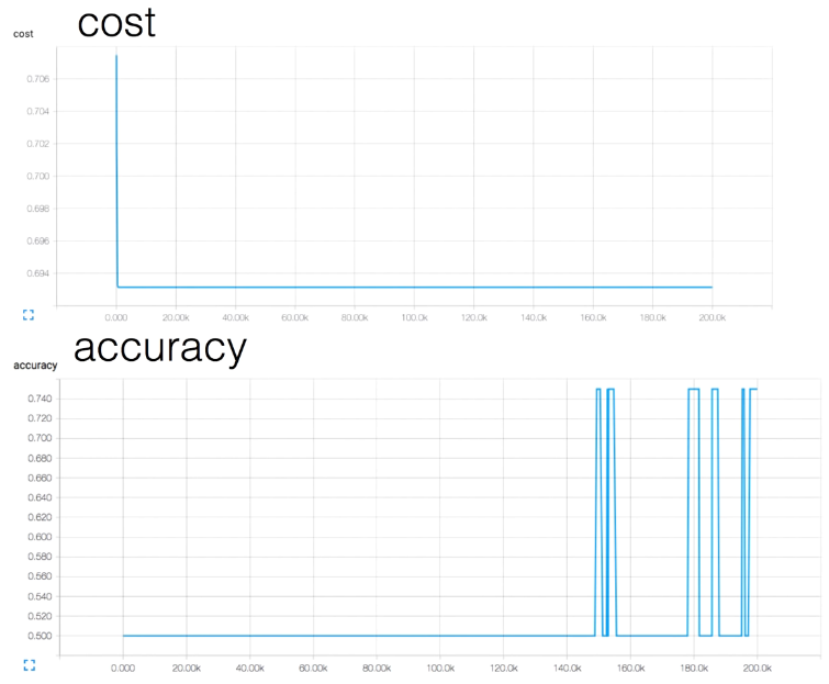
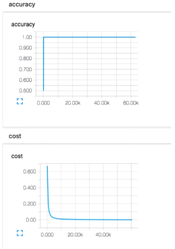
그럼 Accuracy가 높아졌다 낮아졌다를 반복하다가 결국 어떤 수로 유지되고,
cost값은 0에 가까워지는 것이 아닌 0.6에 가까운 값으로 멈춰있는 것을 확인할 수 있다.
왜 이런 현상이 발생하는 것일까?
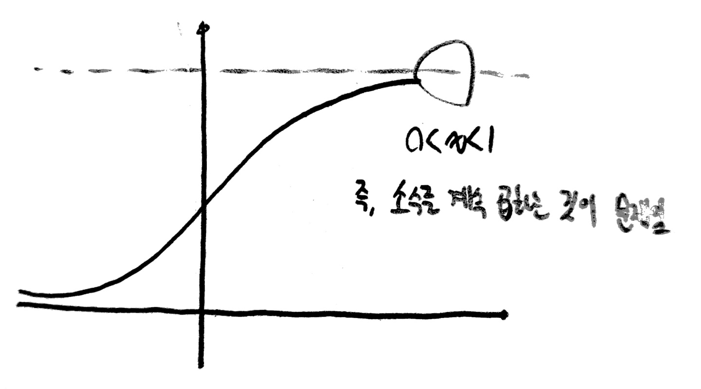
그 이유는 sigmoid의 그래프 모습에 있다.
우리가 이전에 back propagation을 배울 때 확인할 수 있듯이 뒤의 layer의 w, b값을 구하기 위해
앞의 layer에서 사용하는 값들에 대한 미분값들이 필요하다는 점을 알 수 있었다.
그러나 sigmoid함수의 y값은 0~1의 값이기 때문에 반복하여 곱해가면서 그 수가 0에 수렴하게 되고,
앞에 있는 node들의 w, b값 역시 0에 수렴해가면서 변수의 의미를 잃게 되는 것이다.
이를
Vanishing gradient
라고 한다.
이 문제가 앞선 포스팅에서 말했던 [Hinton의 과거 실패한 요인에 대한 고찰 4가지] 중 4번째 문제인
"4. 선형적이지 않은 모습의 공식을 사용함" 이다.
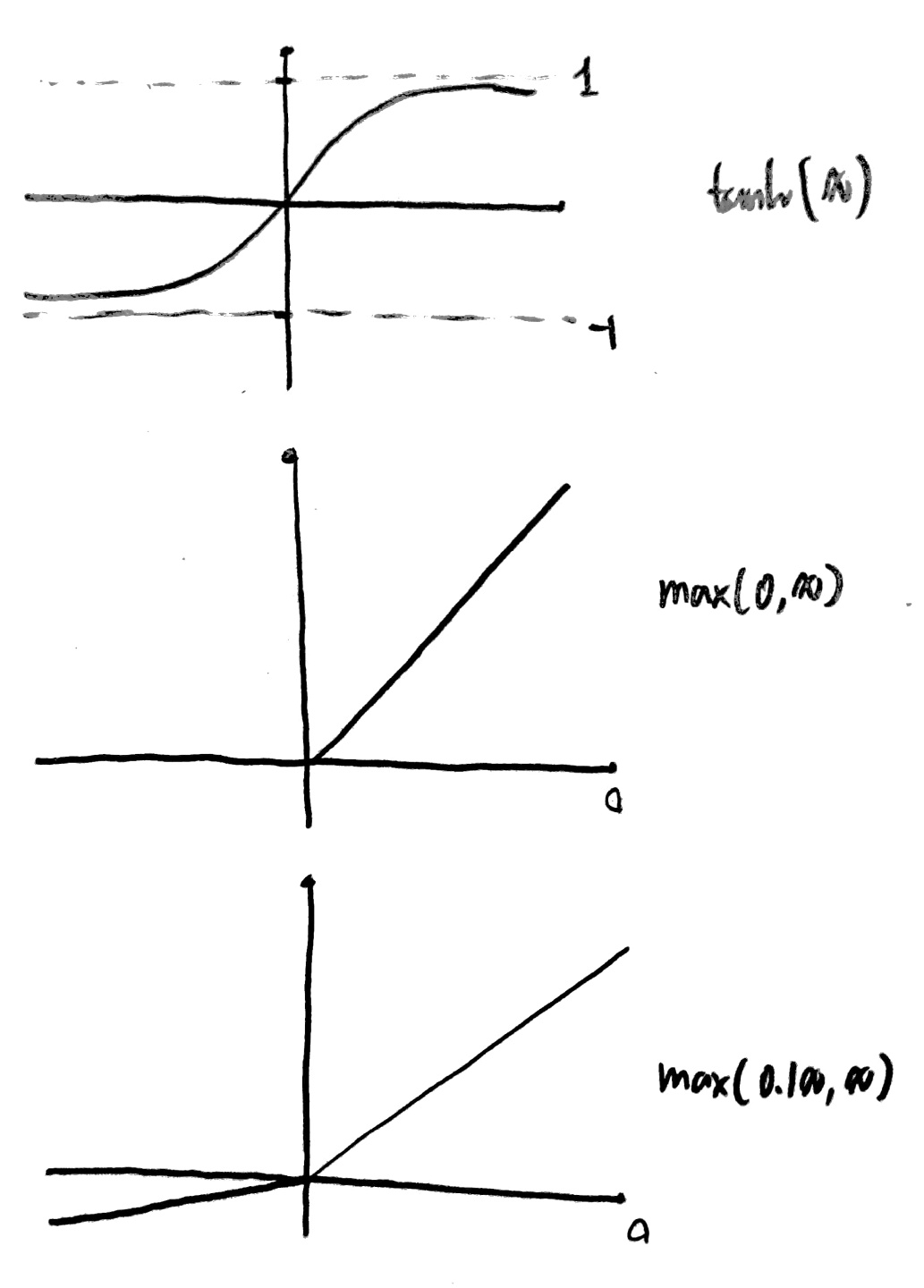
때문에 이를 해결하기 위해 새로운 Activation Function을 사용하기로 했는데 그것이 바로 ReLU 함수이다!
(Rectified Linear Unit)
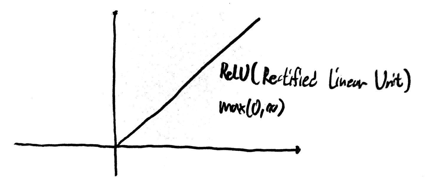
이를 사용하면 Vanishing gradient 문제가 발생하지 않고 학습이 잘 이루어지는 것을 확인할 수 있다.
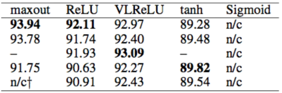
그 외 여러 Activation Function이 존재하고 그 모습은 아래와 같다!
[Weight 초기화 하는 법]
만약 w=0으로 두면 back propagation을 수행하며 앞의 layer에서 사용하는 값이 모두 0이 돼버리는 문제가 발생한다.
때문에 2가지 규칙에 따라 weight값을 구해야함을 Hinton이 제안하였다.
1. 모두 0으로 초기화하지 않는다.
2. RBM구조를 사용하여 학습한다.
(Restricted Boatman Machine)
이때 Restricted는 동일 Layer의 node끼리 연결되지 않았다는 뜻
그럼 RBM이 무엇인지 한번 알아보도록 하자.
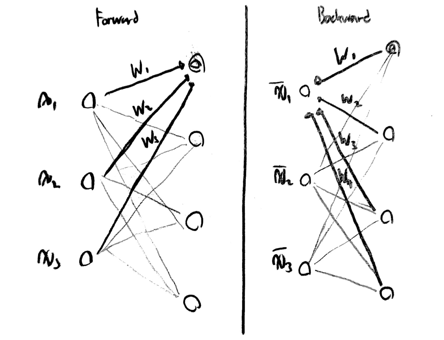
원리 자체는 간단하다.
우선 Forward(encoder라고도 부름) 방향으로 값들을 계산하여 다음 Layer에 결과값을 모두 기입한다.
이후 Backward(decoder라고도 부름)로 다시 값들을 구하면서 새롭게 구한 X 값들을 기입한다.
이때 X값은 X_b라고 하자.
그럼 X-X_b의 차가 최소가 되도록 w값을 조절하면 이것이 RBM의 원리이다.
이때 서로 연결된 2개의 Layer끼리 하나의 RBM을 구성하여 동작한다.
우선 Pre-Training 후 Fine Tuning을 거치면서 w값을 조절하게 된다.
그러나...
RBM을 굳이 사용하지 않아도 된다는 연구결과가 나왔다.
Xavier/He의 초기화 기법으로 적절한 w값을 구할 수 있음을 보였고,
이는 입력값, 출력값(fan_in, fan_out)의 개수에 따라 초기값을 설정하면 된다는 내용의 논문이었다.
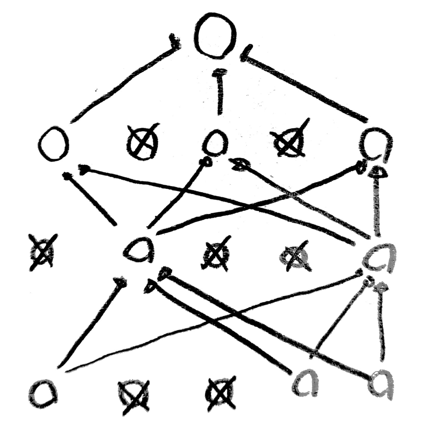
초기화 함수에 따라 정확도가 달라짐 역시 확인할 수 있다.
[Dropout, Ensemble]
우리는 이전 시간에 overfitting의 의미와 이를 방지하기 위한 방법들을 알아보았다.
그 방법들은 아래와 같다.
1. Training data 늘리기
2. feature 줄이기
3. Regularization
이때 Regularization의 경우 regularization strength를 얼마나 주냐에 따라
overfitting을 얼마나 고려해야하는지 알 수 있다고 했다.
그럼 NN을 구축했을 때는 어떻게 Regularization을 수행할 수 있을까?
그 방법에는 Dropout, Ensemble이 있다.
각 방법을 설명하자면 다음과 같다.
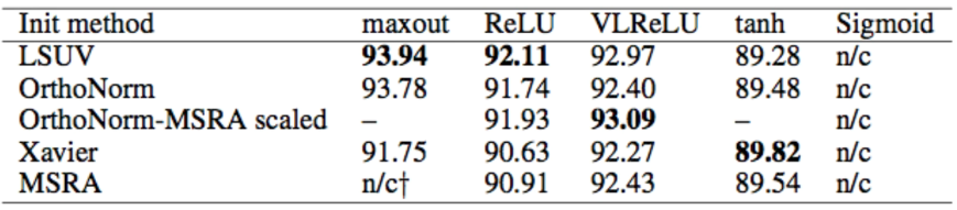
| Dropout | 학습 시 일부 노드들을 죽이는 것이다. 노드를 선택할 때는 랜덤하게 선택하여 죽인다. 이때 판단이나 평가, 판별을 할 때에는 모든 노드들을 사용한다는 것에 유의해야한다. |
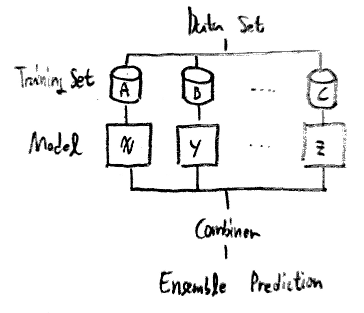
| Ensemble | 여러 모델을 사용하여 결과를 구하고 그 결과를 합하여 결론을 내리는 모델이다. 4%~10%의 성능 향상을 확인할 수 있다. |
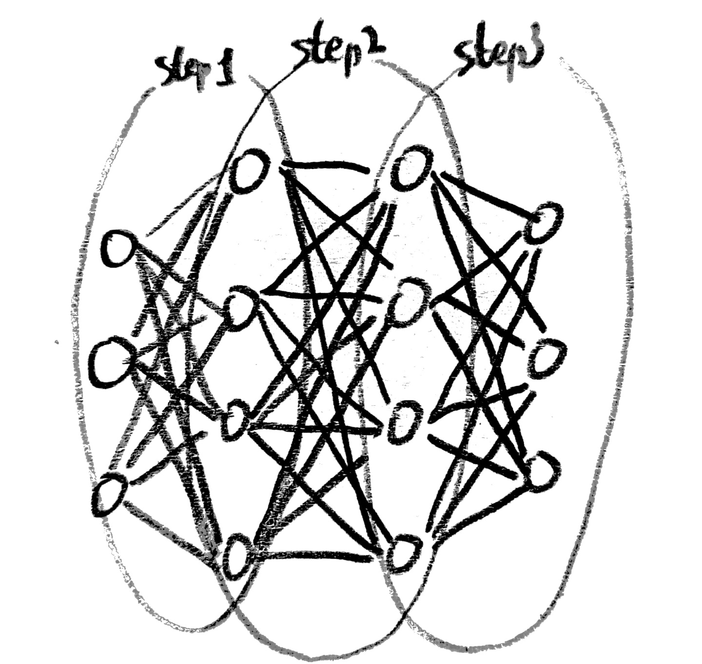
[Make NN using block like Lego]
아래와 같이 다양한 모습의 Network을 형성할 수 있다.
사실... 다음과 같은 모습들은 BoB 경연단계 때 논문에서 많이 보았고, 또 구현도 해봐서 많이 본 친구들이 몇몇 있다!(다 아는 얼굴들이구만!)
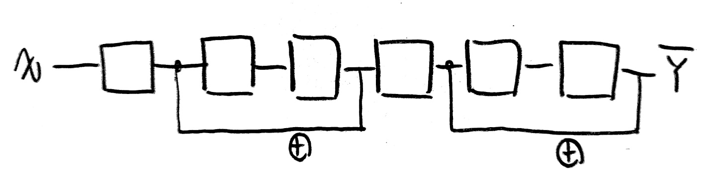
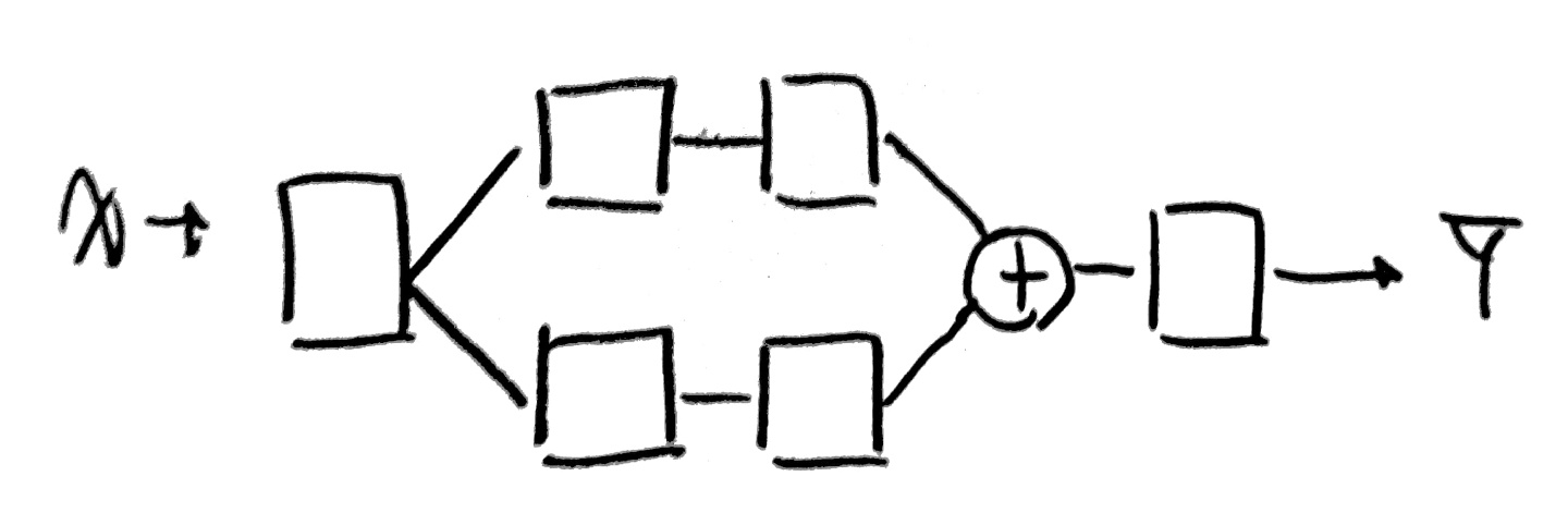
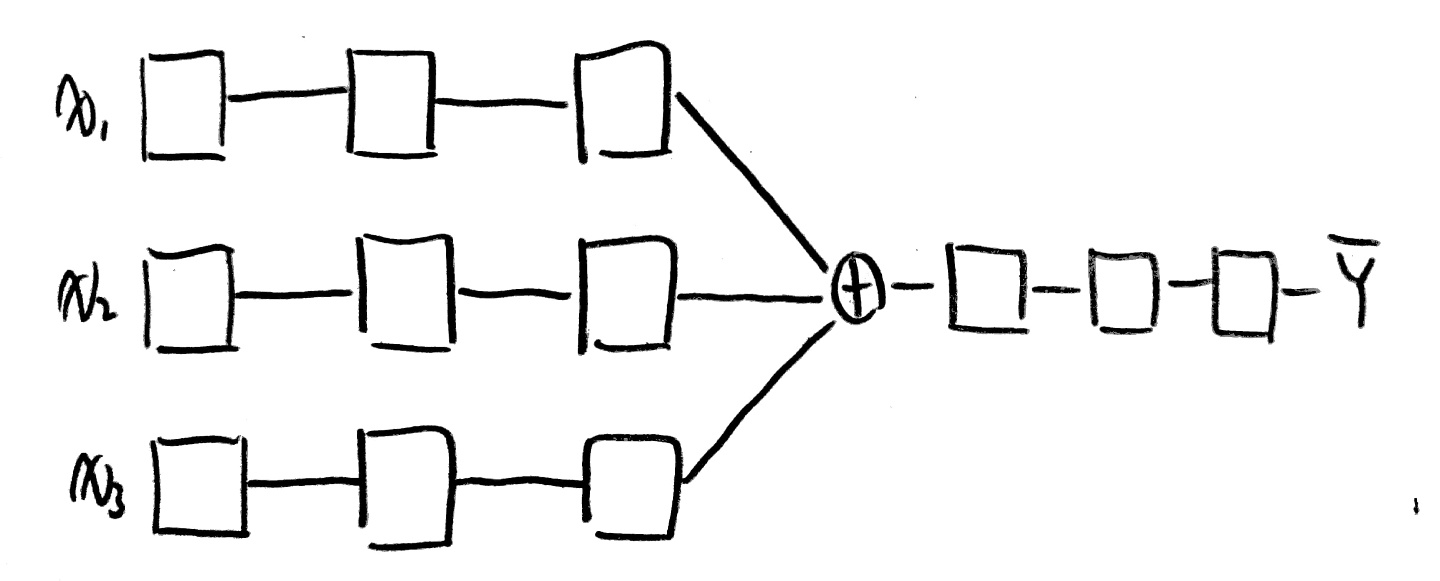
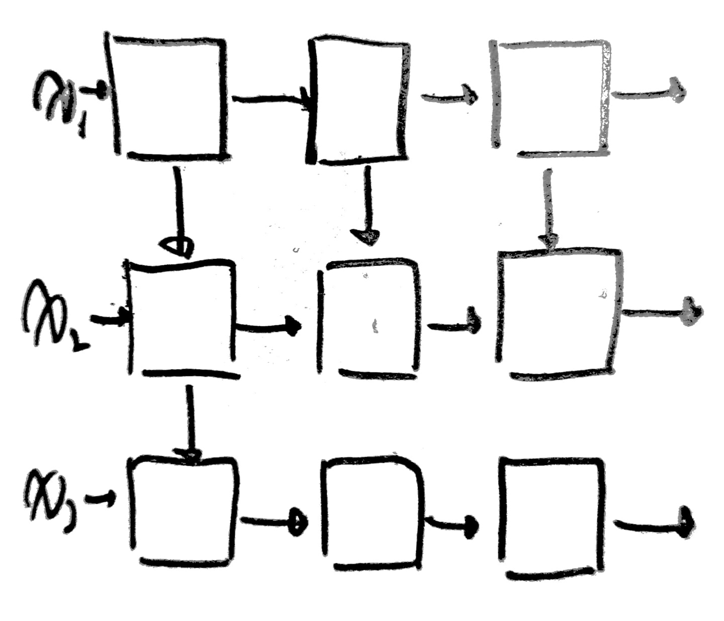
되게되게 다양한 Network 구조를 확인할 수 있다.
'''
NN의 layer를 깊게 구축함으로써 성능 향상을 기대함
약 1%~1.5% 정도의 성능 향상을 확인
'''

import tensorflow.compat.v1 as tf
import matplotlib.pyplot as plt
import numpy as np
import random
tf.disable_v2_behavior()

mnist = tf.keras.datasets.mnist
(x_train, y_train), (x_test, y_test) = mnist.load_data()
# 하나의 행으로 모든 이미지 데이터를 받음
# 60000개의 이미지를 로드함

print(len(x_train), len(y_train), x_train.shape, y_train.shape)
print(len(x_test), len(y_test), x_test.shape, y_test.shape)

x_train, x_test = x_train/255.0, x_test/255.0

nb_classes = 10

#사진 하나당 28*28 픽셀이므로 총 784개의 픽셀임
x_train_new = x_train.reshape(len(x_train), 784)   #60000 * 784 배열로 변경 - 한행당 이미지 하나
y_train_new = np.zeros((len(y_train), nb_classes)) #60000 * 10 배열 생성
for i in range(len(y_train_new)):
    y_train_new[i,y_train[i]] = 1                    #one-hot encoding

x_test_new = x_test.reshape(len(x_test), 784)      #60000 * 784 배열로 변경 - 한행당 이미지 하나
y_test_new = np.zeros((len(y_test), nb_classes))   #60000 * 10 배열 생성
for i in range(len(y_test_new)):
    y_test_new[i,y_test[i]] = 1                      #one-hot encoding

X = tf.placeholder(tf.float32, [None, 784])
Y = tf.placeholder(tf.float32, [None, 10])

W1 = tf.Variable(tf.random_normal([784, 256]))
b1 = tf.Variable(tf.random_normal([256]))
L1 = tf.nn.relu(tf.matmul(X, W1) + b1)

W2 = tf.Variable(tf.random_normal([256, 256]))
b2 = tf.Variable(tf.random_normal([256]))
L2 = tf.nn.relu(tf.matmul(L1, W2) + b2)

W3 = tf.Variable(tf.random_normal([256, 10]))
b3 = tf.Variable(tf.random_normal([10]))
hypothesis = tf.matmul(L2, W3) + b3

cost = tf.reduce_mean(tf.nn.softmax_cross_entropy_with_logits(logits=hypothesis, labels=Y))
optimizer = tf.train.AdamOptimizer(learning_rate=0.001).minimize(cost)

is_correct = tf.equal(tf.arg_max(hypothesis, 1), tf.arg_max(Y, 1))
accuracy = tf.reduce_mean(tf.cast(is_correct, tf.float32))

# parameters
training_epochs = 15
batch_size = 100
total_batch = int(len(x_train_new) / batch_size)

with tf.Session() as sess:
    sess.run(tf.global_variables_initializer())
    for epoch in range(training_epochs):
        avg_cost = 0

        for i in range(total_batch):
            batch_xs = x_train_new[(epoch * batch_size):(epoch + 1) * batch_size]
            batch_ys = y_train_new[(epoch * batch_size):(epoch + 1) * batch_size]

            _, cost_val = sess.run([optimizer, cost], feed_dict={X: batch_xs, Y: batch_ys})
            avg_cost += cost_val / total_batch

        print("Epoch: {:04d}, Cost: {:.9f}".format(epoch + 1, avg_cost))

    print("Accuracy: ", accuracy.eval(session=sess, feed_dict={X: x_test_new, Y: y_test_new}))

    random_idx = random.randrange(1, 10000)
    print ("random_idx : ", random_idx)
    print("Prediction: ", sess.run(tf.argmax(hypothesis, 1), feed_dict={X: x_test_new[random_idx : random_idx + 1]}))

    plt.imshow(
        x_test_new[random_idx : random_idx + 1].reshape(28, 28),
        cmap="Greys",
        interpolation="nearest",
    )
    plt.show()
'''
w값의 적절한 초기화로 모델 성능이 향상됨
'''

import tensorflow.compat.v1 as tf
import matplotlib.pyplot as plt
import numpy as np
import random
tf.disable_v2_behavior()

mnist = tf.keras.datasets.mnist
(x_train, y_train), (x_test, y_test) = mnist.load_data()
# 하나의 행으로 모든 이미지 데이터를 받음
# 60000개의 이미지를 로드함

print(len(x_train), len(y_train), x_train.shape, y_train.shape)
print(len(x_test), len(y_test), x_test.shape, y_test.shape)

x_train, x_test = x_train/255.0, x_test/255.0

nb_classes = 10

#사진 하나당 28*28 픽셀이므로 총 784개의 픽셀임
x_train_new = x_train.reshape(len(x_train), 784)   #60000 * 784 배열로 변경 - 한행당 이미지 하나
y_train_new = np.zeros((len(y_train), nb_classes)) #60000 * 10 배열 생성
for i in range(len(y_train_new)):
    y_train_new[i,y_train[i]] = 1                    #one-hot encoding

x_test_new = x_test.reshape(len(x_test), 784)      #60000 * 784 배열로 변경 - 한행당 이미지 하나
y_test_new = np.zeros((len(y_test), nb_classes))   #60000 * 10 배열 생성
for i in range(len(y_test_new)):
    y_test_new[i,y_test[i]] = 1                      #one-hot encoding

X = tf.placeholder(tf.float32, [None, 784])
Y = tf.placeholder(tf.float32, [None, 10])

#initializer=tf.contrib.layers.xavier_initializer()
init = tf.truncated_normal_initializer(stddev=0.1)

W1 = tf.get_variable("W1", shape=[784, 256], initializer=init)
b1 = tf.Variable(tf.random_normal([256]))
L1 = tf.nn.relu(tf.matmul(X, W1) + b1)

W2 = tf.get_variable("W2", shape=[256, 256], initializer=init)
b2 = tf.Variable(tf.random_normal([256]))
L2 = tf.nn.relu(tf.matmul(L1, W2) + b2)

W3 = tf.get_variable("W3", shape=[256, 10], initializer=init)
b3 = tf.Variable(tf.random_normal([10]))
hypothesis = tf.matmul(L2, W3) + b3

cost = tf.reduce_mean(tf.nn.softmax_cross_entropy_with_logits(logits=hypothesis, labels=Y))
optimizer = tf.train.AdamOptimizer(learning_rate=0.001).minimize(cost)

is_correct = tf.equal(tf.arg_max(hypothesis, 1), tf.arg_max(Y, 1))
accuracy = tf.reduce_mean(tf.cast(is_correct, tf.float32))

# parameters
training_epochs = 15
batch_size = 100
total_batch = int(len(x_train_new) / batch_size)

with tf.Session() as sess:
    sess.run(tf.global_variables_initializer())
    for epoch in range(training_epochs):
        avg_cost = 0

        for i in range(total_batch):
            batch_xs = x_train_new[(epoch * batch_size):(epoch + 1) * batch_size]
            batch_ys = y_train_new[(epoch * batch_size):(epoch + 1) * batch_size]

            _, cost_val = sess.run([optimizer, cost], feed_dict={X: batch_xs, Y: batch_ys})
            avg_cost += cost_val / total_batch

        print("Epoch: {:04d}, Cost: {:.9f}".format(epoch + 1, avg_cost))

    print("Accuracy: ", accuracy.eval(session=sess, feed_dict={X: x_test_new, Y: y_test_new}))

    random_idx = random.randrange(1, 10000)
    print ("random_idx : ", random_idx)
    print("Prediction: ", sess.run(tf.argmax(hypothesis, 1), feed_dict={X: x_test_new[random_idx : random_idx + 1]}))

    plt.imshow(
        x_test_new[random_idx : random_idx + 1].reshape(28, 28),
        cmap="Greys",
        interpolation="nearest",
    )
    plt.show()
'''
만약 dropout이 없다면
모델이 overfitting되어 학습의 효과가 눈에 띄게 보이지 않음
때문에 dropout을 통해 몇몇 node를 죽임으로써
효과적인 학습이 가능하도록 함
(이때 반드시 평가 및 예측 시에는 keep_prob값을 1로 줌으로써 모든 node를 사용하도록 함)
'''

import tensorflow.compat.v1 as tf
import matplotlib.pyplot as plt
import numpy as np
import random
tf.disable_v2_behavior()

mnist = tf.keras.datasets.mnist
(x_train, y_train), (x_test, y_test) = mnist.load_data()
# 하나의 행으로 모든 이미지 데이터를 받음
# 60000개의 이미지를 로드함

print(len(x_train), len(y_train), x_train.shape, y_train.shape)
print(len(x_test), len(y_test), x_test.shape, y_test.shape)

x_train, x_test = x_train/255.0, x_test/255.0

nb_classes = 10

#사진 하나당 28*28 픽셀이므로 총 784개의 픽셀임
x_train_new = x_train.reshape(len(x_train), 784)   #60000 * 784 배열로 변경 - 한행당 이미지 하나
y_train_new = np.zeros((len(y_train), nb_classes)) #60000 * 10 배열 생성
for i in range(len(y_train_new)):
    y_train_new[i,y_train[i]] = 1                    #one-hot encoding

x_test_new = x_test.reshape(len(x_test), 784)      #60000 * 784 배열로 변경 - 한행당 이미지 하나
y_test_new = np.zeros((len(y_test), nb_classes))   #60000 * 10 배열 생성
for i in range(len(y_test_new)):
    y_test_new[i,y_test[i]] = 1                      #one-hot encoding

X = tf.placeholder(tf.float32, [None, 784])
Y = tf.placeholder(tf.float32, [None, 10])

#initializer=tf.contrib.layers.xavier_initializer()
init = tf.truncated_normal_initializer(stddev=0.1)
keep_prob = tf.placeholder(tf.float32)

W1 = tf.get_variable("W1", shape=[784, 512], initializer=init)
b1 = tf.Variable(tf.random_normal([512]))
L1 = tf.nn.relu(tf.matmul(X, W1) + b1)
L1 = tf.nn.dropout(L1, keep_prob=keep_prob)

W2 = tf.get_variable("W2", shape=[512, 512], initializer=init)
b2 = tf.Variable(tf.random_normal([512]))
L2 = tf.nn.relu(tf.matmul(L1, W2) + b2)
L2 = tf.nn.dropout(L2, keep_prob=keep_prob)

W3 = tf.get_variable("W3", shape=[512, 512], initializer=init)
b3 = tf.Variable(tf.random_normal([512]))
L3 = tf.nn.relu(tf.matmul(L2, W3) + b3)
L3 = tf.nn.dropout(L3, keep_prob=keep_prob)

W4 = tf.get_variable("W4", shape=[512, 512], initializer=init)
b4 = tf.Variable(tf.random_normal([512]))
L4 = tf.nn.relu(tf.matmul(L3, W4) + b4)
L4 = tf.nn.dropout(L4, keep_prob=keep_prob)

W5 = tf.get_variable("W5", shape=[512, 10], initializer=init)
b5 = tf.Variable(tf.random_normal([10]))
hypothesis = tf.matmul(L4, W5) + b5

cost = tf.reduce_mean(tf.nn.softmax_cross_entropy_with_logits(logits=hypothesis, labels=Y))
optimizer = tf.train.AdamOptimizer(learning_rate=0.001).minimize(cost)

is_correct = tf.equal(tf.arg_max(hypothesis, 1), tf.arg_max(Y, 1))
accuracy = tf.reduce_mean(tf.cast(is_correct, tf.float32))

# parameters
training_epochs = 15
batch_size = 100
total_batch = int(len(x_train_new) / batch_size)

with tf.Session() as sess:
    sess.run(tf.global_variables_initializer())
    for epoch in range(training_epochs):
        avg_cost = 0

        for i in range(total_batch):
            batch_xs = x_train_new[(epoch * batch_size):(epoch + 1) * batch_size]
            batch_ys = y_train_new[(epoch * batch_size):(epoch + 1) * batch_size]

            _, cost_val = sess.run([optimizer, cost], feed_dict={X: batch_xs, Y: batch_ys, keep_prob: 0.7})
            avg_cost += cost_val / total_batch

        print("Epoch: {:04d}, Cost: {:.9f}".format(epoch + 1, avg_cost))

    print("Accuracy: ", accuracy.eval(session=sess, feed_dict={X: x_test_new, Y: y_test_new, keep_prob: 1}))

    random_idx = random.randrange(1, 10000)
    print ("random_idx : ", random_idx)
    print("Prediction: ", sess.run(tf.argmax(hypothesis, 1), feed_dict={X: x_test_new[random_idx : random_idx + 1], keep_prob: 1}))

    plt.imshow(
        x_test_new[random_idx : random_idx + 1].reshape(28, 28),
        cmap="Greys",
        interpolation="nearest",
    )
plt.show()'AI > 모두를 위한 딥러닝 정리' 카테고리의 다른 글
| Day12. Recurrent Neural Network (0) | 2022.04.21 |
|---|---|
| Day11. Convolution Neural Network (0) | 2022.04.21 |
| Day9. Neural Network and TensorBoard code (0) | 2022.04.19 |
| Day8. Basic information for Neural Network (0) | 2022.04.18 |
| Day7. learning rate, overfitting, regularization (0) | 2022.04.16 |


댓글