드디어 본격적으로 Neural Network(이하 NN)를 공부한다.
일단 미리 말해두지만 선형대수, 통계학 지식이 없는 나는 그냥 수박겉핥기로 공부하는 거다...
저 두 지식은 BoB에서 만났던, 좋은 인연이 되주신 형님이 알려준 커리큘럼대로 공부해볼 예정이다.
(Kaggle master가 알려준 방법이니... 효과적이겠지?)
그럼 이제 시작해보자!
[NN의 구현]
저번 시간에 우리는 XOR 문제를 하나의 Perceptron으로 해결할 수 없다는 것을 볼 수 있었다.
(뒤에 나오는 코드를 실행시켜보면 실제로 해결되지 않는 것을 확인할 수 있음)
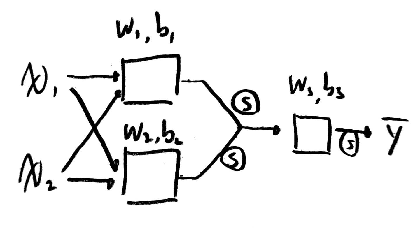
때문에 아래 사진과 같은 NN을 구성해야한다!
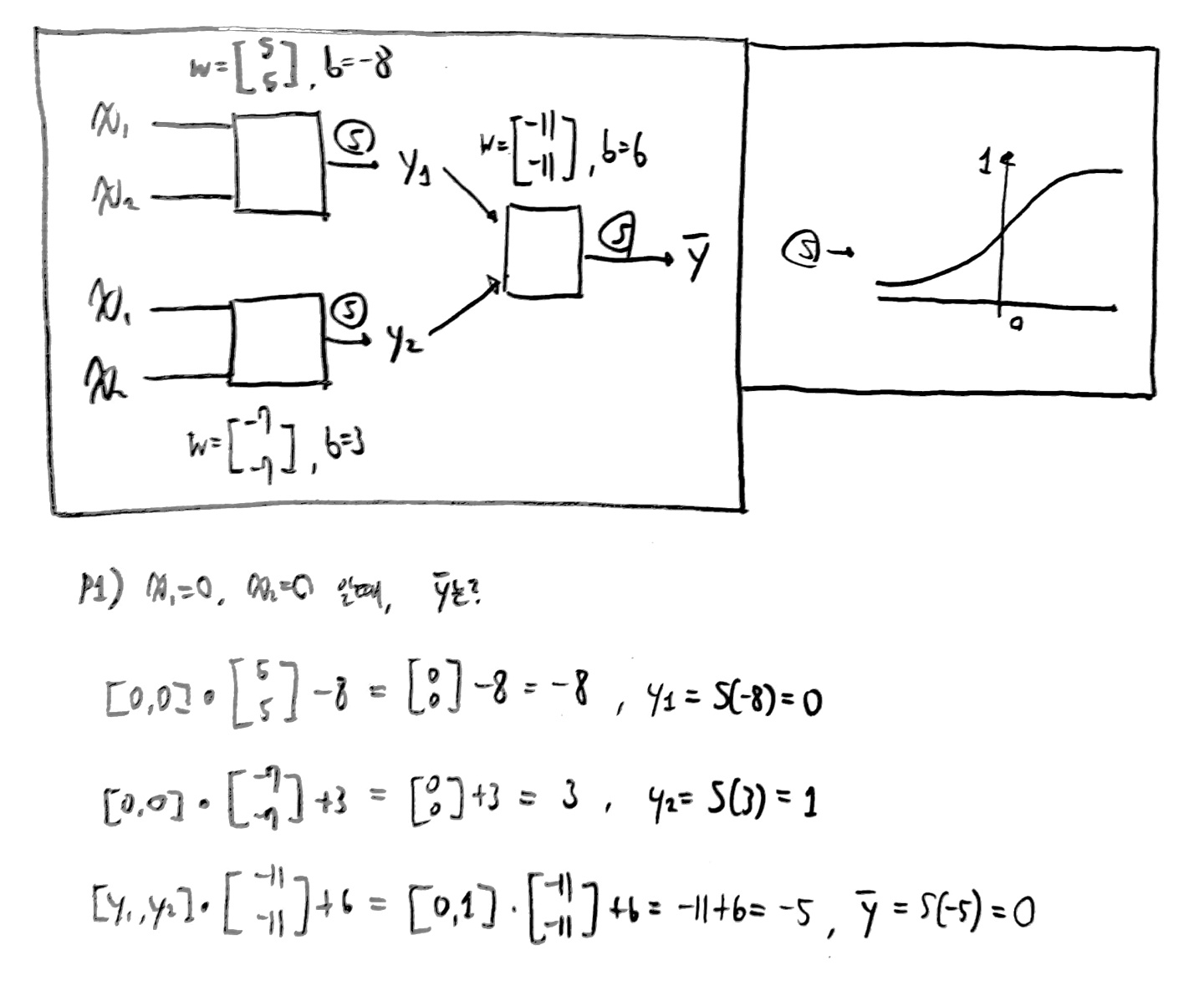
아래의 풀이 과정대로 (x1, x2)에 (0, 1), (1, 0), (1, 1)을 대입하여 풀이하면 다음과 같은 결과가 나온다.
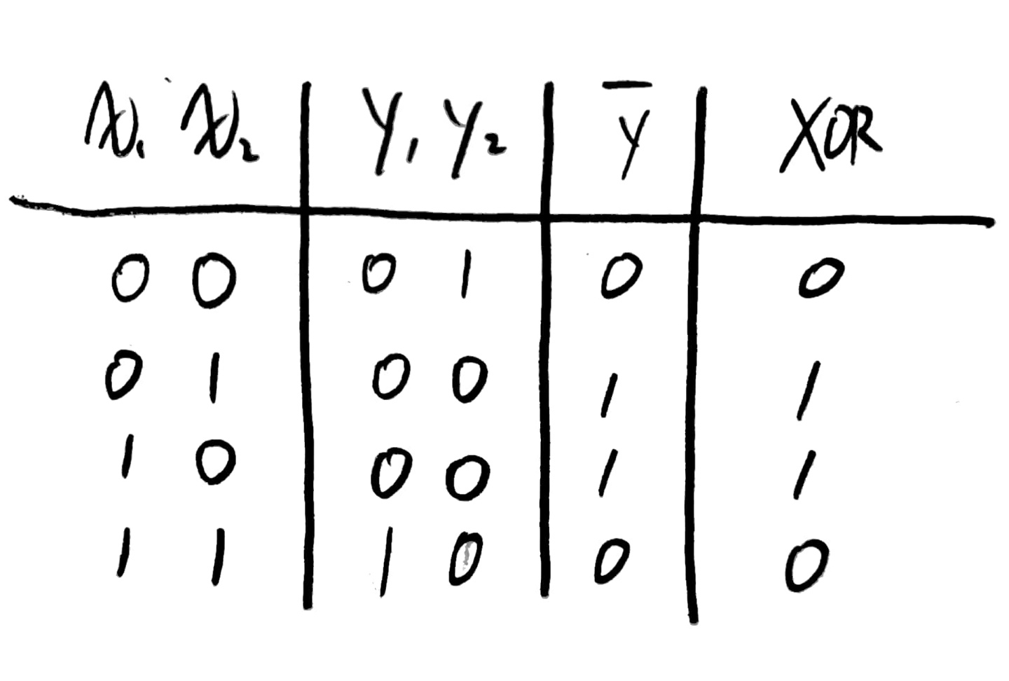
즉, 하나의 Perceptron으로 구성된 네트워크에서는 해결이 불가능했지만,
2개 이상의 Perceptron으로 구성된 네트워크에서는 해결이 가능하다는 것을 알 수 있다!
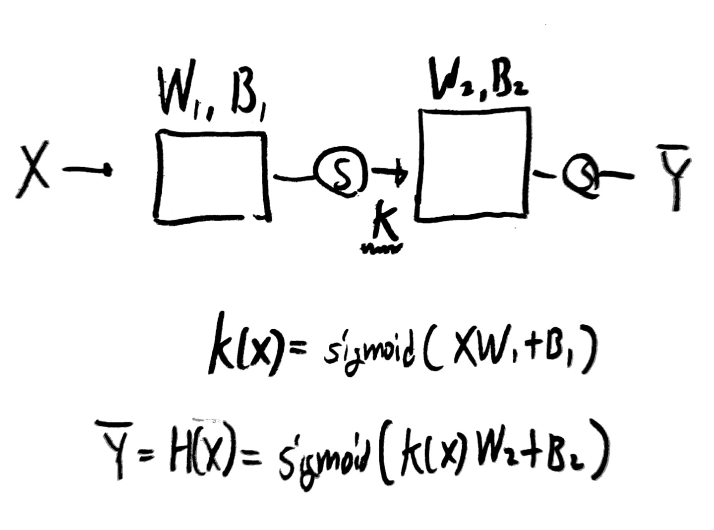
실제 구현시 여러 perceptron을 하나의 행렬로 묶어 표현할 수 있으므로 코드 상으로 표현하기도 매우 간단할 것 같다!
[간단한 편미분 지식]
편미분은 어떤 함수에서 하나의 변수가 그 함수에 미치는 변화율이 어느정도인지 알 수 있도록 해주는 도구이다!
때문에 변화율을 알고 싶은 하나의 변수를 선택했다면,
나머지 변수들은 상수 취급하여 미분하면 그것이 편미분을 하는 방법이다.
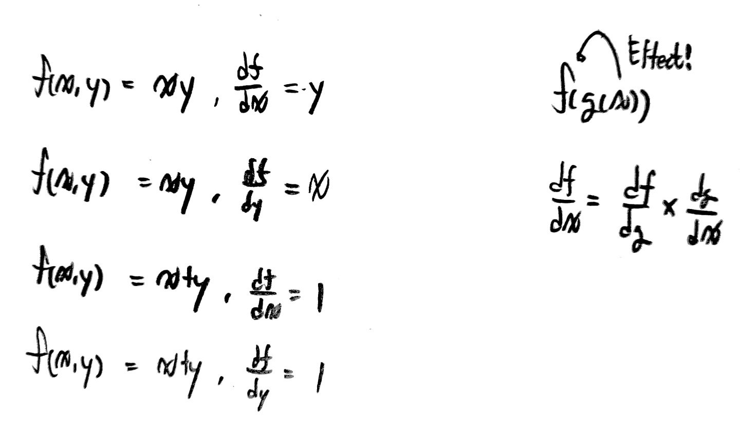
[Back Propagation의 원리]
back Propagation의 원리를 알아보기 위해 상황을 가정하여 back propagation을 적용해보자.
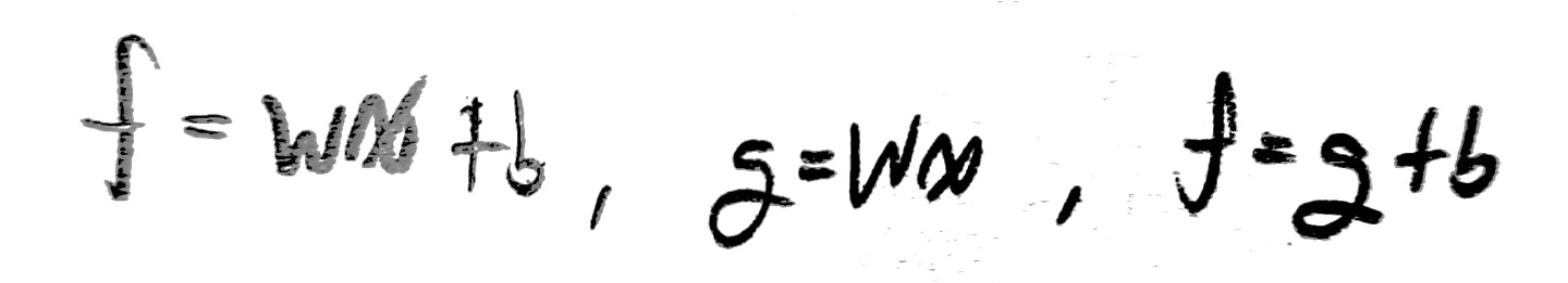
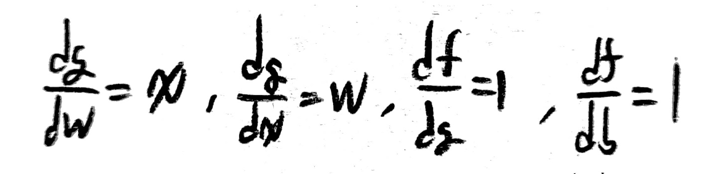
위 상황은 w=-2, x=5, b=3, f=-7인 상황을 가정하고 구한 각 변수들의 값이다.
저 값들을 구하는 것은 그렇게 어렵지 않지만, 중요한 것은 저 값들이 가지는 의미를 이해하는 것이다.
미분한 값들은 모두 이러한 형태를 지닌다.
df/dx
아까 말했듯이 이 말의 의미는 x가 f의 값을 결정하는대 미치는 변화율을 의미한다.
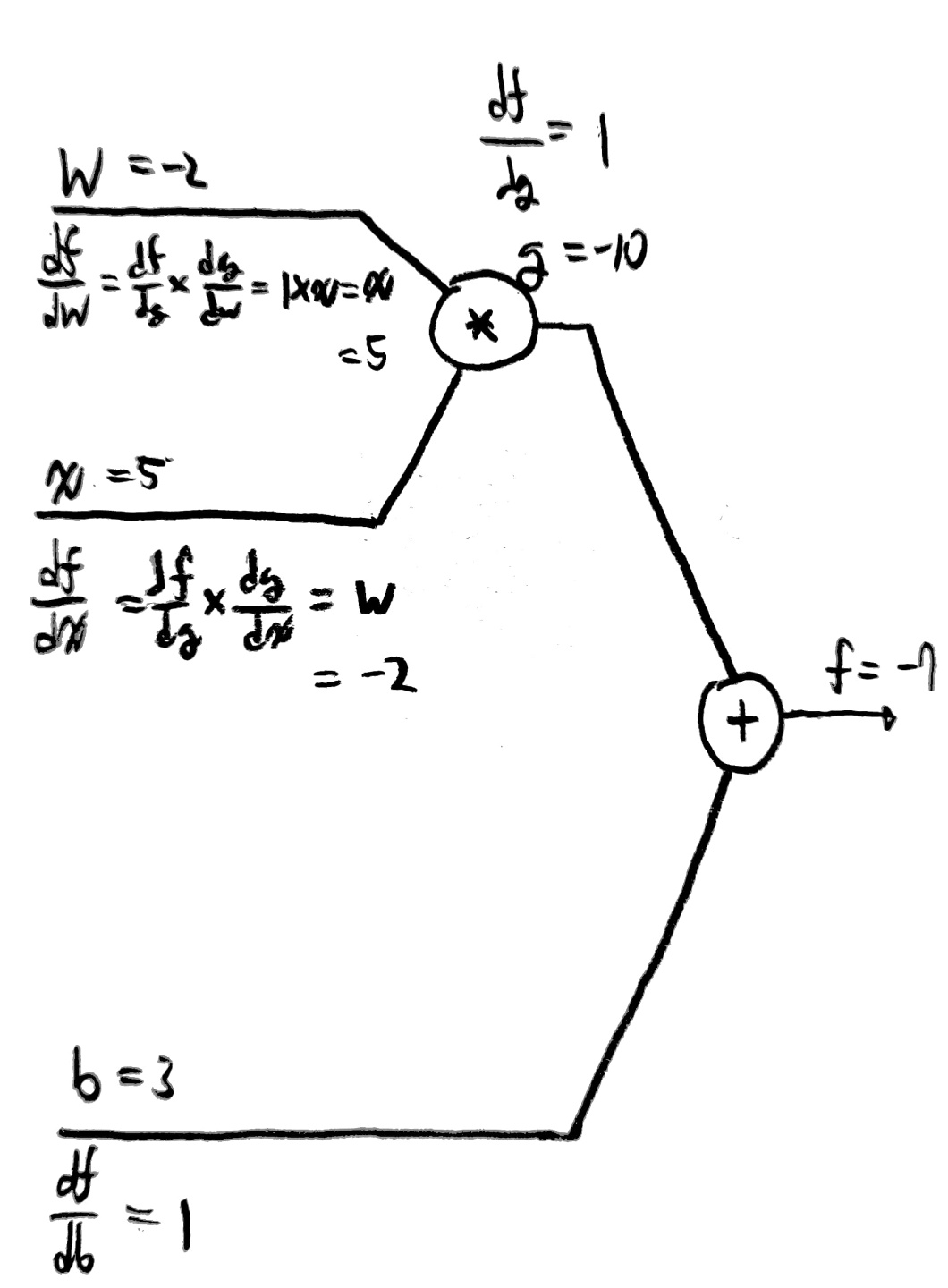
때문에 위 그래프에서 df/dx의 값이 -2라는 뜻은 x가 1씩 변화할 때마다 f는 -2씩 변화하게 된다는 뜻이다.
실제로 f = wx + b이므로 f = -2x + 3임을 알 수 있고 x가 1씩 변화할 때마다 f가 -2만큼 변화한다는 것을 알 수 있다!
그럼 이 지식을 가지고 각 변수가 학습 결과에 미치는 영향을 정말 구할 수 있는가가 궁금할 것이다.
아래 사진을 보자.
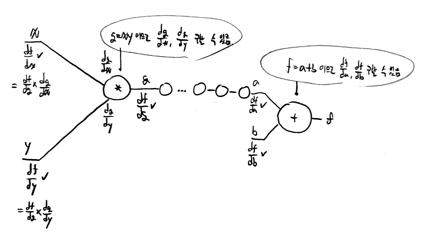
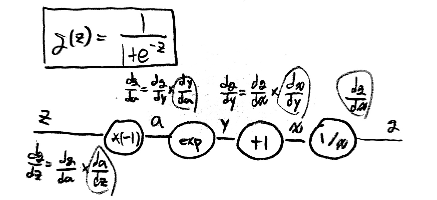
위 그림에서 볼 수 있듯이 연산의 종류를 알고 있고 입력값, 출력값, hypothesis를 모두 알고 있기 때문에
결과값(f)을 가지고 뒤에서부터 차례대로 모든 값들을 추측할 수 있다는 것이다.
(직접 위 사진을 따라가면 이해가 쉬울 것임)
이를 통해 우리는 Back propagation을 통해 어떻게 올바른 w, b값을 NN에서 구할 수 있는지 알 수 있었고,
동시에 복잡한 NN이 구축될수록 올바른 w, b를 구하는데 오랜 시간이 걸릴 수 있다는 것을 알 수 있었다.
'''
XOR 문제를 해결하지 못함
'''
import tensorflow.compat.v1 as tf
tf.disable_v2_behavior()
import numpy as np

x_data = np.array([[0, 0], [0, 1], [1, 0], [1, 1]], dtype=np.float32)
y_data = np.array([[0], [1], [1], [0]], dtype=np.float32)

X = tf.placeholder(tf.float32)
Y = tf.placeholder(tf.float32)
W = tf.Variable(tf.random_normal([2, 1]), name="weight")
b = tf.Variable(tf.random_normal([1]), name="bias")
hypothesis = tf.sigmoid(tf.matmul(X, W) + b)

cost = -tf.reduce_mean(Y * tf.log(hypothesis) + (1 - Y) * tf.log(1 - hypothesis))
train = tf.train.GradientDescentOptimizer(learning_rate=0.1).minimize(cost)

predicted = tf.cast(hypothesis > 0.5, dtype=tf.float32)
accuracy = tf.reduce_mean(tf.cast(tf.equal(predicted, Y), dtype=tf.float32))

with tf.Session() as sess:
    sess.run(tf.global_variables_initializer())

    for step in range(15001):
        sess.run(train, feed_dict={X: x_data, Y: y_data})
        if step % 100 == 0:
            print(step, sess.run(cost, feed_dict={X: x_data, Y: y_data}), sess.run(W))

    h, c, a = sess.run([hypothesis, predicted, accuracy], feed_dict={X: x_data, Y: y_data})
    print("\nHypothesis: ", h, "\nCorrect: ", c, "\nAccuracy: ", a)
'''
NN을 사용하여 XOR 문제를 해결할 수 있음
'''
import tensorflow.compat.v1 as tf
tf.disable_v2_behavior()
import numpy as np

x_data = np.array([[0, 0], [0, 1], [1, 0], [1, 1]], dtype=np.float32)
y_data = np.array([[0], [1], [1], [0]], dtype=np.float32)
X = tf.placeholder(tf.float32)
Y = tf.placeholder(tf.float32)

#NN을 위한 layer의 구분
#만약 wide한 NN을 구축하고 싶다면 아래 코드를 다음과 같이 변경해야함
'''
W1 = tf.Variable(tf.random_normal([2,10]), name='weight1')
b1 = tf.Variable(tf.random_normal([10]), name='bias1')
layer1 = tf.sigmoid(tf.matmul(X, W1) + b1)
W2 = tf.Variable(tf.random_normal([10,1]), name='weight2')
b2 = tf.Variable(tf.random_normal([1]), name='bias2')
hypothesis = tf.sigmoid(tf.matmul(layer1, W2) + b2)
'''
#만약 Deep한 NN을 구축하고 싶다면 아래 코드를 다음과 같이 변경해야함
'''
W1 = tf.Variable(tf.random_normal([2,10]), name='weight1')
b1 = tf.Variable(tf.random_normal([10]), name='bias1')
layer1 = tf.sigmoid(tf.matmul(X, W1) + b1)
W2 = tf.Variable(tf.random_normal([10,10]), name='weight2')
b2 = tf.Variable(tf.random_normal([10]), name='bias2')
layer2 = tf.sigmoid(tf.matmul(layer1, W2) + b2)
W3 = tf.Variable(tf.random_normal([10,10]), name='weight3')
b3 = tf.Variable(tf.random_normal([10]), name='bias3')
layer3 = tf.sigmoid(tf.matmul(layer2, W3) + b3)
W4 = tf.Variable(tf.random_normal([10,1]), name='weight4')
b4 = tf.Variable(tf.random_normal([1]), name='bias4')
hypothesis = tf.sigmoid(tf.matmul(layer3, W4) + b4)
'''
W1 = tf.Variable(tf.random_normal([2,2]), name='weight1')
b1 = tf.Variable(tf.random_normal([2]), name='bias1')
layer1 = tf.sigmoid(tf.matmul(X, W1) + b1)
W2 = tf.Variable(tf.random_normal([2,1]), name='weight2')
b2 = tf.Variable(tf.random_normal([1]), name='bias2')
hypothesis = tf.sigmoid(tf.matmul(layer1, W2) + b2)

cost = -tf.reduce_mean(Y * tf.log(hypothesis) + (1 - Y) * tf.log(1 - hypothesis))
train = tf.train.GradientDescentOptimizer(learning_rate=0.1).minimize(cost)

predicted = tf.cast(hypothesis > 0.5, dtype=tf.float32)
accuracy = tf.reduce_mean(tf.cast(tf.equal(predicted, Y), dtype=tf.float32))

with tf.Session() as sess:
    sess.run(tf.global_variables_initializer())

    for step in range(15001):
        sess.run(train, feed_dict={X: x_data, Y: y_data})
        if step % 100 == 0:
            print(step, sess.run(cost, feed_dict={X: x_data, Y: y_data}), sess.run([W1, W2]))

    h, c, a = sess.run([hypothesis, predicted, accuracy], feed_dict={X: x_data, Y: y_data})
    print("\nHypothesis: ", h, "\nCorrect: ", c, "\nAccuracy: ", a)
[TensorBoard를 사용하기 위한 순서]
- 로깅하고 싶은 tensor를 결정한다.
- 모든 summary들을 Merge한다.
- writer를 생성하고 graph를 add한다.
- summary merge와 add_summary를 실행한다.
- TersorBoard를 실행한다(명령어를 통해 실행할 수 있음).
import tensorflow.compat.v1 as tf
tf.disable_v2_behavior()
import numpy as np

x_data = np.array([[0, 0], [0, 1], [1, 0], [1, 1]], dtype=np.float32)
y_data = np.array([[0], [1], [1], [0]], dtype=np.float32)
X = tf.placeholder(tf.float32, [None, 2], name="x")
Y = tf.placeholder(tf.float32, [None, 1], name="y")

#그래프를 그릴때 layer1, layer2를 구분하여 그려줌
#with name_scope로 구분하지 않으면 모든 node가 한꺼번에 노출됨
with tf.name_scope("Layer1"):
    W1 = tf.Variable(tf.random_normal([2, 2]), name="weight1")
    b1 = tf.Variable(tf.random_normal([2]), name="bias1")
    layer1 = tf.sigmoid(tf.matmul(X, W1) + b1)

    tf.summary.histogram("W1", W1)
    tf.summary.histogram("b1", b1)
    tf.summary.histogram("Layer1", layer1)


with tf.name_scope("Layer2"):
    W2 = tf.Variable(tf.random_normal([2, 1]), name="weight2")
    b2 = tf.Variable(tf.random_normal([1]), name="bias2")
    hypothesis = tf.sigmoid(tf.matmul(layer1, W2) + b2)

    tf.summary.histogram("W2", W2)
    tf.summary.histogram("b2", b2)
    tf.summary.histogram("Hypothesis", hypothesis)
    #여러 값에 대한 logging함수인 histogram

with tf.name_scope("Cost"):
    cost = -tf.reduce_mean(Y * tf.log(hypothesis) + (1 - Y) * tf.log(1 - hypothesis))
    tf.summary.scalar("Cost", cost) #하나의 값에 대한 logging함수인 scalar

with tf.name_scope("Train"):
    train = tf.train.AdamOptimizer(learning_rate=0.01).minimize(cost)

predicted = tf.cast(hypothesis > 0.5, dtype=tf.float32)
accuracy = tf.reduce_mean(tf.cast(tf.equal(predicted, Y), dtype=tf.float32))
tf.summary.scalar("accuracy", accuracy)

# 그래프로 시각화 실행
with tf.Session() as sess:
    merged_summary = tf.summary.merge_all()
    writer = tf.summary.FileWriter("./logs/xor_logs_r0_01") #logging 정보를 저장할 dir경로
    writer.add_graph(sess.graph)  # 그래프 실행

    sess.run(tf.global_variables_initializer())

    for step in range(10001):
        _, summary, cost_val = sess.run([train, merged_summary, cost], feed_dict={X: x_data, Y: y_data})
        # global_step이 그래프에서 하나의 축을 차지하게 됨(횟수를 변수로 둠)
        writer.add_summary(summary, global_step=step)

        if step % 100 == 0:
            print(step, cost_val)

    h, p, a = sess.run([hypothesis, predicted, accuracy], feed_dict={X: x_data, Y: y_data})
print(f"\nHypothesis:\n{h} \nPredicted:\n{p} \nAccuracy:\n{a}")'AI > 모두를 위한 딥러닝 정리' 카테고리의 다른 글
| Day11. Convolution Neural Network (0) | 2022.04.21 |
|---|---|
| Day10. Activation Functions, weight initialization, Dropout and Ensemble (0) | 2022.04.20 |
| Day8. Basic information for Neural Network (0) | 2022.04.18 |
| Day7. learning rate, overfitting, regularization (0) | 2022.04.16 |
| Day6. Softmax (0) | 2022.04.11 |


댓글