<Multinomial Classification>
이번에 공부한 내용은 Y의 종류가 여러 개 존재하는 상황에서의 분류이다.
이전까지는 powerpoint에 그림을 그려서 붙여 넣었지만 이제는 직접 쓰고 이것을 스캔하여 사용하도록 하겠다!
(절대로 powerpoint 사용이 귀찮아서가 아니다...ㅎㅎ)
우선 다음과 같은 데이터가 있다고 가정하자.
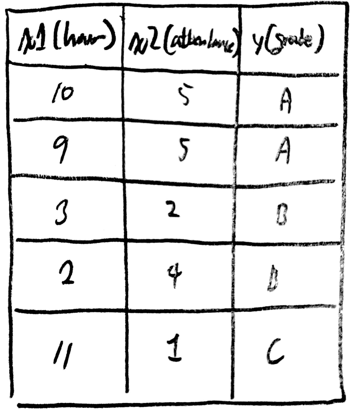
데이터를 보면 2개의 독립변수가 Y의 종속변수로써 사용되는 상황임을 알 수 있다.
이때, 중요한 것은 여러 변수가 존재하면 여러 차원으로 나타난다는 점에 유의해야한다.
위와 같이 변수의 개수가 3개인 경우 3차원에서 면으로 만들어진 식이 주어지게 될 것이라는 점이 중요하다.
(이게 헷갈려서 고생 조금 했다... 수학 못하는 나란 녀석...)
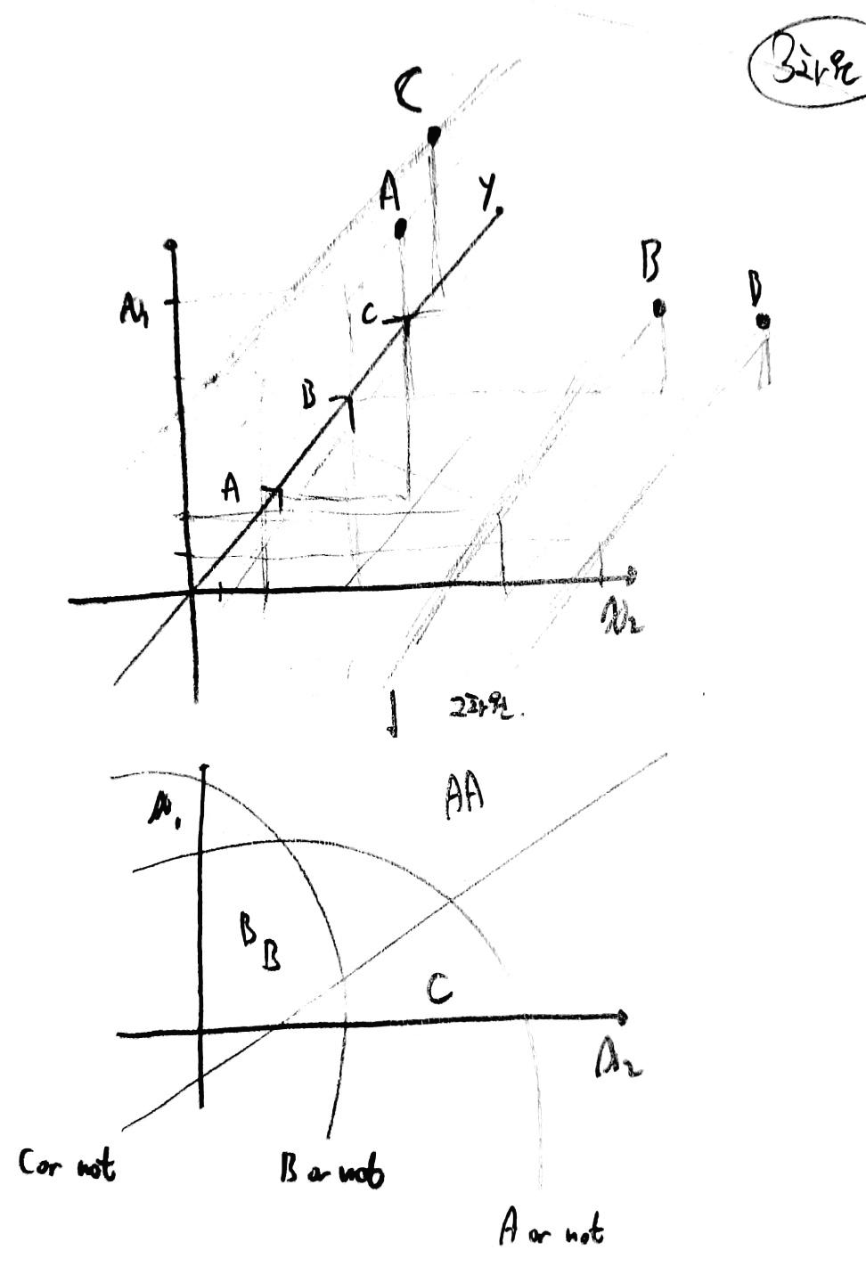
즉, 3차원 그래프에서 나타나는 면으로 이뤄진 식을 잘라 2차원으로 표현한 모습이다.
그럼 2개 이상의 변수가 다차원의 그래프를 형성하고
(x 변수가 다양해질 수록 고차원의 그래프 형성)
이러한 상황을 학습하면 각 X1, X2에 맞는 가중치가 생성된다.
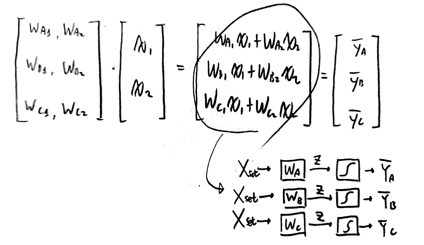
x값이 독립변수이기 때문에 각 변수가 지니는 가중치는 당연히 다를 수 밖에 없고 그로 인해
여러 가중치 값들이 도출될 수 밖에 없다.
그럼 도출된 가중치 행렬을 x변수 행렬과 곱해 각 a, b, c의 결과값(확률 아님)을 얻을 수 있다.
하지만 우리가 원하는 것은 아래와 같이 합이 1이 되는 a, b, c일 확률을 구하고 싶다.
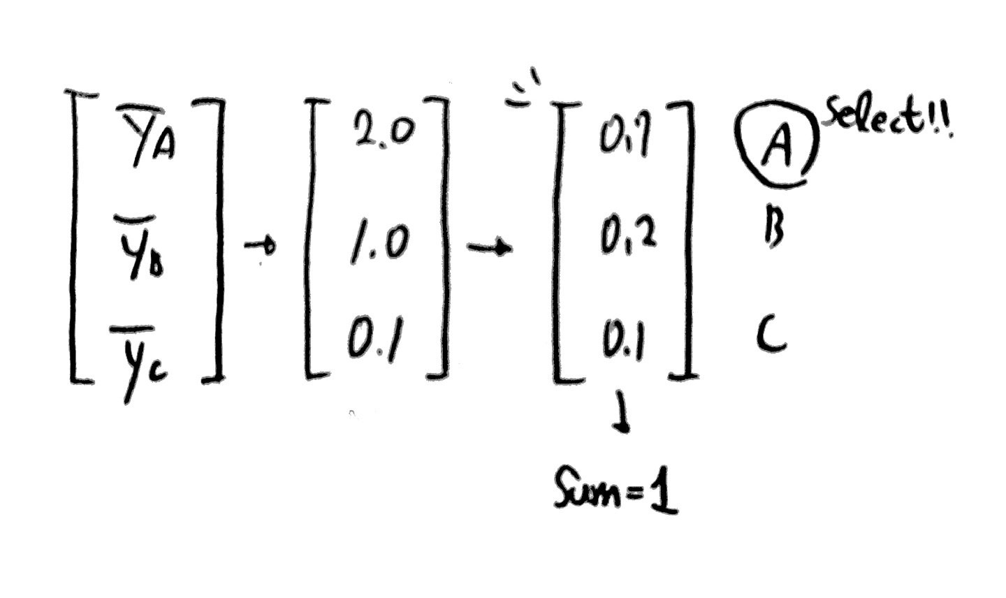
이때 우리가 SOFTMAX 함수를 사용하게 된다!
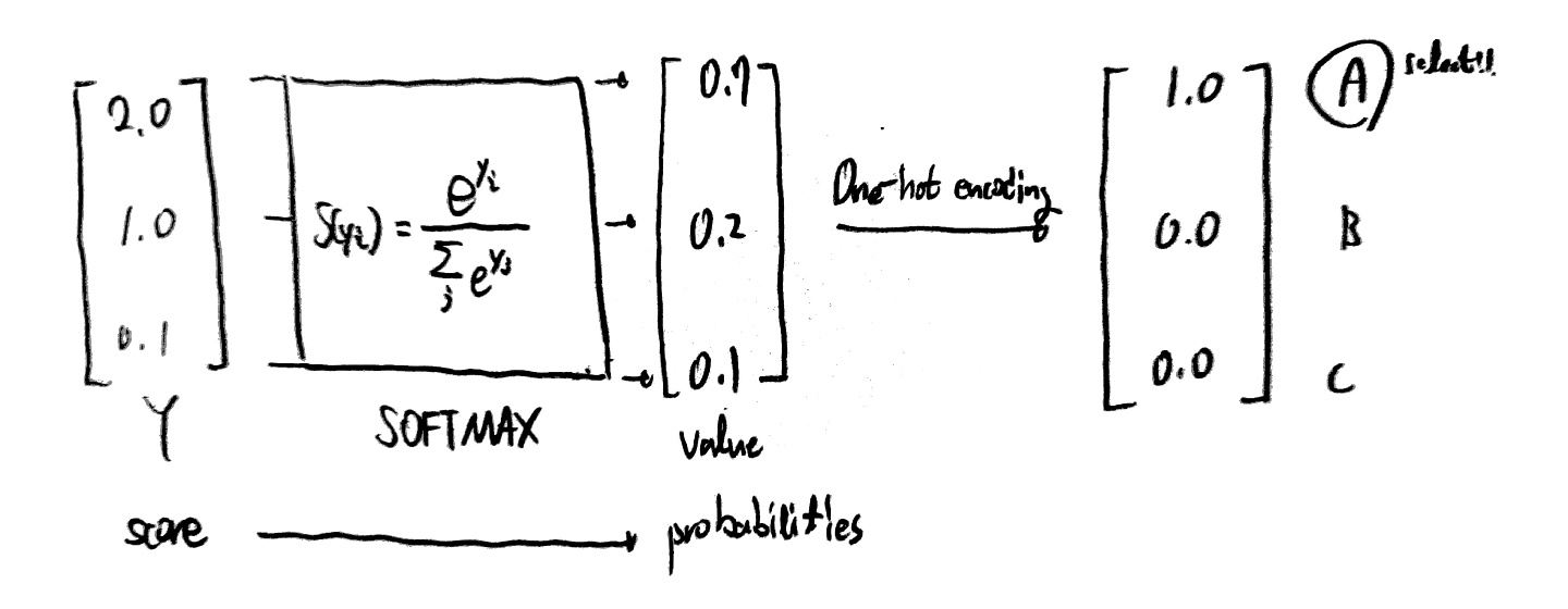
위와 같은 과정을 거쳐 우리가 원하는 multinomial classification이 가능하게 된다.
이때 One-Hot encoding이 무엇이냐!
그냥 0, 1로 어떤 데이터이느냐를 구분하도록 해주는 것이 one-hot encoding이다.
별거 없어...
<Multinomial Classification's Cost Function>
이제 cost function에 대해 알아보자.
Y값은 모두 예측했으니 이제 모델의 성능을 향상 시키기 위해 가중치를 수정하는 과정을 거칠 것이다.
이를 위해 사용되는 cost function은 다음과 같다.
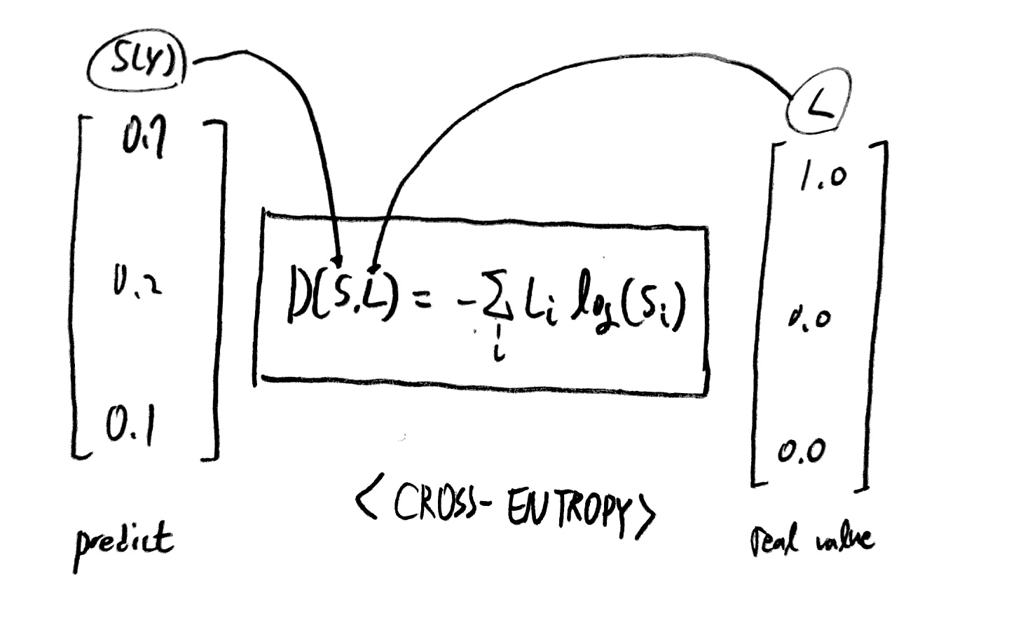

다음과 같은 함수를 cost function으로 사용한다.
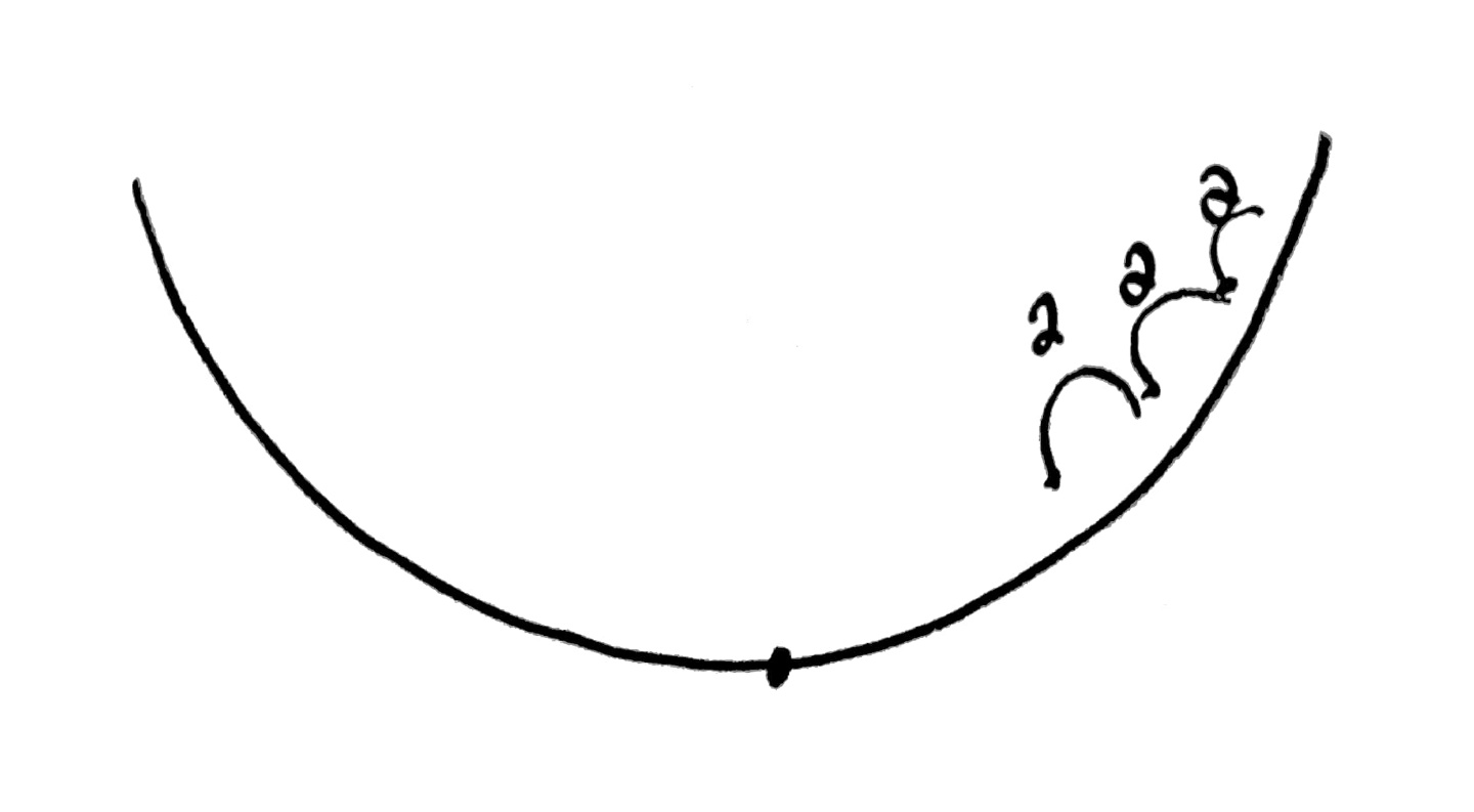
수학적 지식은 우선 밀어두고,
절대 이렇게 해선 안된다, 나는 인공지능 응애 레벨이라 빠르게 공부하기 위해 이렇게하지,
원래는 cost function이 왜 저런식으로 나타나는 지에 대해서도 면밀히 공부해야한다.
위 손실 함수를 통해 실제로 사용 가능한 함수인지 알아보도록 하자.
위와 같이 우리가 원하는 대로 작동하는 손실 함수가 된다는 것을 알 수 있다.
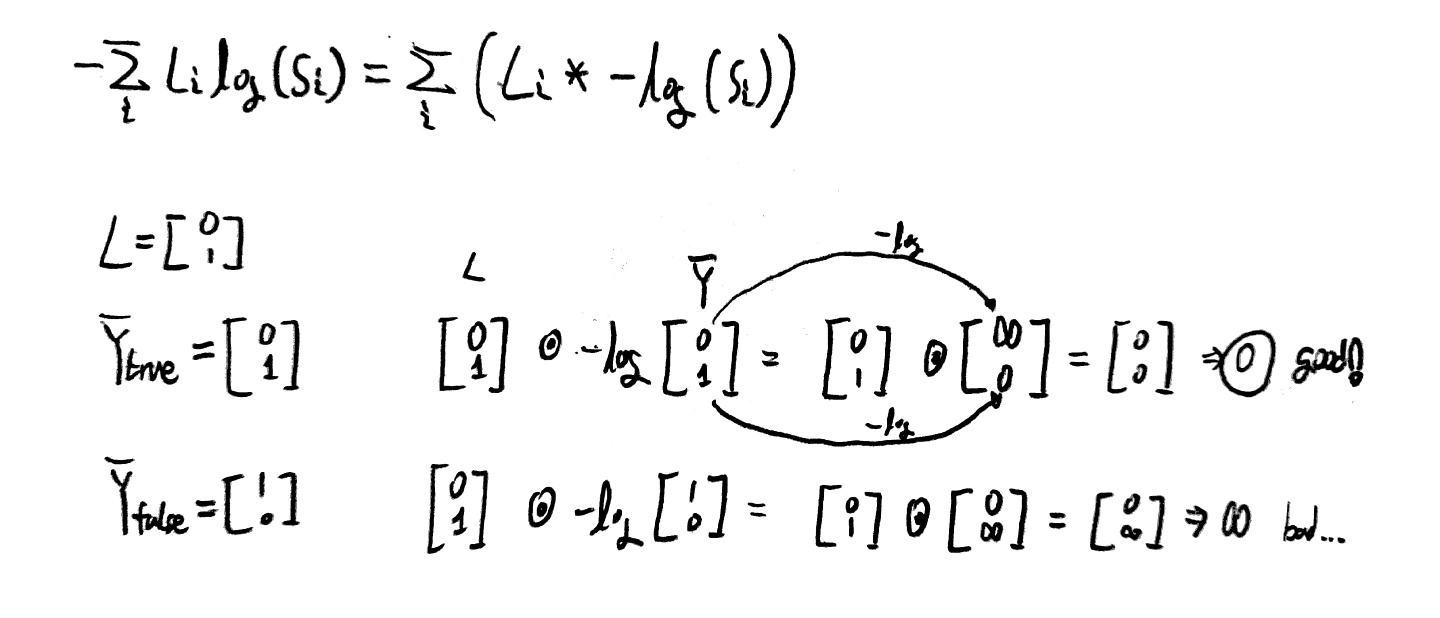
좀 더 자세히 설명하자면, Y_true값을 주고 식을 전개했을 때
손실이 0으로 나오므로 옳은 판별이라 말할 수 있고(모델이 옳음),
Y_false를 주고 식을 전개했을 때
손실이 무한수가 나오므로 이 또한 옳은 판별임을 알 수 있다(모델이 옳음).
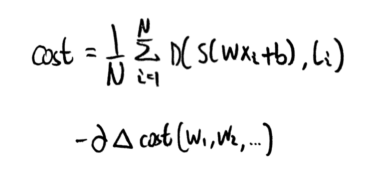
정리하자면 cost function과 이를 미분한 식의 모습은 아래와 같고
Gradient descent를 하기에 좋은 모습이라는 점도 알 수 있다.
import tensorflow.compat.v1 as tf
tf.disable_v2_behavior()

x_data = [[1, 2, 1, 1],
          [2, 1, 3, 2],
          [3, 1, 3, 4],
          [4, 1, 5, 5],
          [1, 7, 5, 5],
          [1, 2, 5, 6],
          [1, 6, 6, 6],
          [1, 7, 7, 7]]

y_data = [[0, 0, 1],
          [0, 0, 1],
          [0, 0, 1],
          [0, 1, 0],
          [0, 1, 0],
          [0, 1, 0],
          [1, 0, 0],
          [1, 0, 0]]

X = tf.placeholder("float", [None, 4])
Y = tf.placeholder("float", [None, 3])
nb_classes = 3

W = tf.Variable(tf.random_normal([4, nb_classes]), name='weight')
b = tf.Variable(tf.random_normal([nb_classes]), name='bias')

hypothesis = tf.nn.softmax(tf.matmul(X, W) + b)

# Cross entropy
cost = tf.reduce_mean(-tf.reduce_sum(Y * tf.log(hypothesis), axis=1))

optimizer = tf.train.GradientDescentOptimizer(learning_rate=0.1).minimize(cost)

# Launch graph
with tf.Session() as sess:
    sess.run(tf.global_variables_initializer())

    for step in range(2001):
            _, cost_val = sess.run([optimizer, cost], feed_dict={X: x_data, Y: y_data})

            if step % 200 == 0:
                print(step, cost_val)

    #arg_max를 통해 결과로 도출된 리스트안의 몇 번째 값이 가장 높은지 반환해줌
    print('--------------')
    a = sess.run(hypothesis, feed_dict={X: [[1, 11, 7, 9]]})
    print(a, sess.run(tf.arg_max(a, 1))) #B

    print('--------------')
    b = sess.run(hypothesis, feed_dict={X: [[1, 3, 4, 3]]})
    print(b, sess.run(tf.arg_max(b, 1))) #A

    print('--------------')
    c = sess.run(hypothesis, feed_dict={X: [[1, 1, 0, 1]]})
    print(c, sess.run(tf.arg_max(c, 1))) #C

    print('--------------')
    all = sess.run(hypothesis, feed_dict={X: [[1, 11, 7, 9], [1, 3, 4, 3], [1, 1, 0, 1]]})
    print(all, sess.run(tf.arg_max(all, 1)))
import numpy as np
import tensorflow.compat.v1 as tf
tf.disable_v2_behavior()

# Predicting animal type based on various features
xy = np.loadtxt('data.csv', delimiter=',', dtype=np.float32)
x_data = xy[:, 0:-1]
y_data = xy[:, [-1]]
print(x_data.shape, y_data.shape)

nb_classes = 7  # 0 ~ 6

X = tf.placeholder(tf.float32, [None, 16])
Y = tf.placeholder(tf.int32, [None, 1])  # 0 ~ 6

'''
one_hot: Tensor("one_hot:0", shape=(?, 1, 7), dtype=float32)
reshape one_hot: Tensor("Reshape:0", shape=(?, 7), dtype=float32)
'''
#shape->(?, 1, 7) 이건 우리가 원하던 결과의 모습이 아님
Y_one_hot = tf.one_hot(Y, nb_classes)
#shape->(?, 7)의 형태로 reshape를 해줌으로써 원하던 결과의 모습을 얻음
Y_one_hot = tf.reshape(Y_one_hot, [-1, nb_classes])

W = tf.Variable(tf.random_normal([16, nb_classes]), name='weight')
b = tf.Variable(tf.random_normal([nb_classes]), name='bias')

logits = tf.matmul(X, W) + b
hypothesis = tf.nn.softmax(logits)

# Cross entropy cost/loss
cost_i = tf.nn.softmax_cross_entropy_with_logits(logits=logits, labels=Y_one_hot)
cost = tf.reduce_mean(cost_i)
optimizer = tf.train.GradientDescentOptimizer(learning_rate=0.1).minimize(cost)

prediction = tf.argmax(hypothesis, 1)
correct_prediction = tf.equal(prediction, tf.argmax(Y_one_hot, 1))
accuracy = tf.reduce_mean(tf.cast(correct_prediction, tf.float32))

# Launch graph
with tf.Session() as sess:
    sess.run(tf.global_variables_initializer())
    for step in range(2001):
        _, cost, acc = sess.run([optimizer, cost, accuracy], feed_dict={X: x_data, Y: y_data})
        if step % 100 == 0:
            print("Step: {:5}\tCost: {:.3f}\tAcc: {:.2%}".format(step, cost, acc))

    pred = sess.run(prediction, feed_dict={X: x_data})
    for p, y in zip(pred, y_data.flatten()):
print("[{}] Prediction: {} True Y: {}".format(p == int(y), p, int(y)))'AI > 모두를 위한 딥러닝 정리' 카테고리의 다른 글
| Day8. Basic information for Neural Network (0) | 2022.04.18 |
|---|---|
| Day7. learning rate, overfitting, regularization (0) | 2022.04.16 |
| Day5. Logistic Classification과 Logistic Regression (0) | 2022.04.01 |
| Day4. multi-variable linear regression (0) | 2022.03.21 |
| Day3. Gradient descent algorithm (0) | 2022.03.05 |


댓글