[Overshooting]
overshooting은 learning rate의 크기에 따라 학습에 대한 가중치를 찾을 수 없게 되는 현상을 의미한다.
1. learning rate가 너무 클 경우
사진과 같이 cost값이 너무 커지거나 가장 작은 cost 값을 구하지 못해,
잘못된 가중치를 반환할 수 있다.
이를 해결하기 위해 cost값을 출력해보며 값이 너무 커지거나 숫자가 아닌 이상한 값들이 출력될 경우,
learning rate를 줄여가며 학습 후 결과를 살펴본다.
2. learning rate가 너무 작을 경우
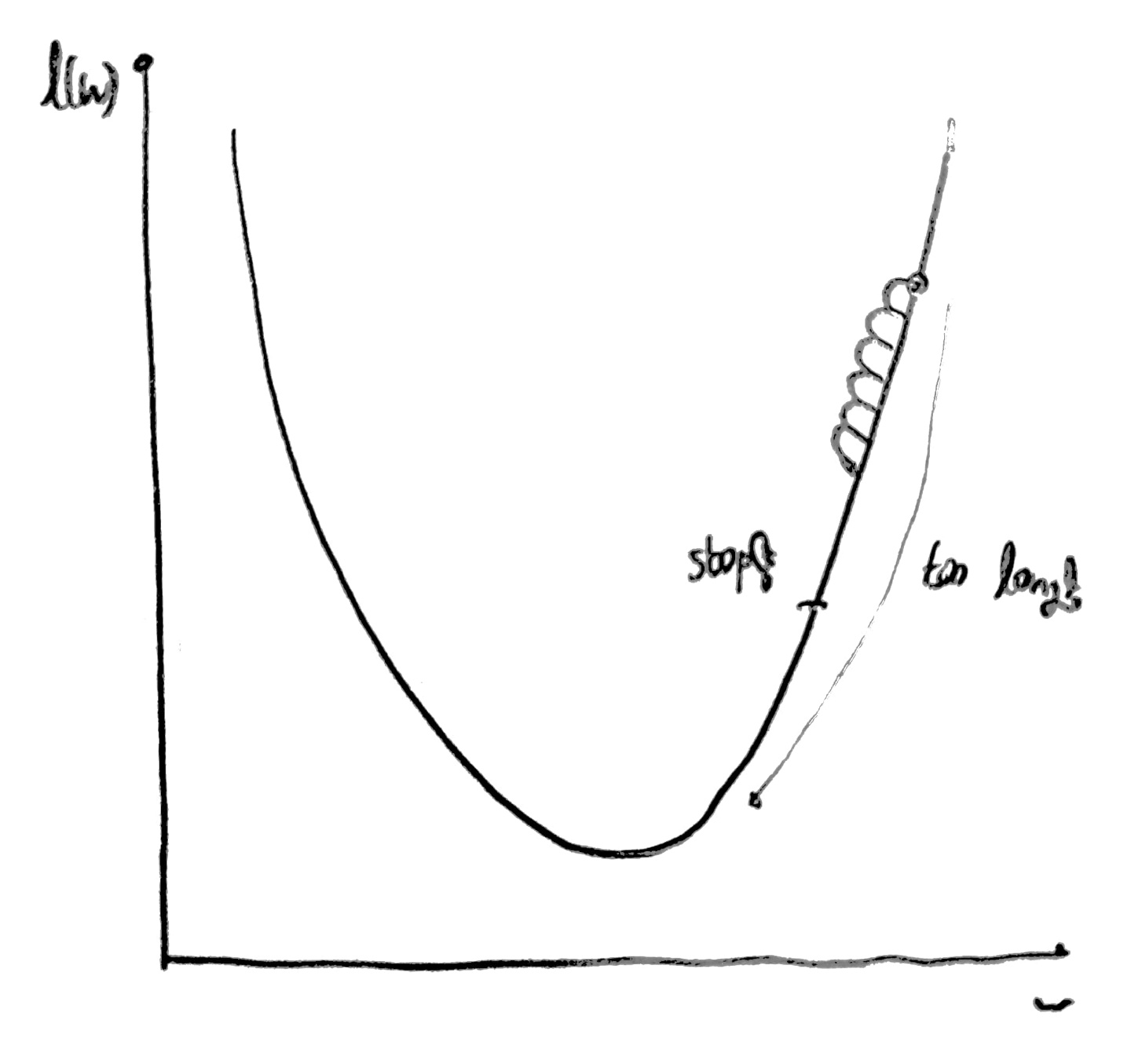
사진과 같이 cost 값이 너무 작게 변화하여 가장 작은 cost 값을 구하지 못해,
잘못된 가중치를 반환할 수 있다.
이를 해결하기 위해 cost값을 출력해보며 값이 너무 작게 변화하면 learning rate값을 증가시킨 후,
다시 학습시켜 결과를 살펴본다.
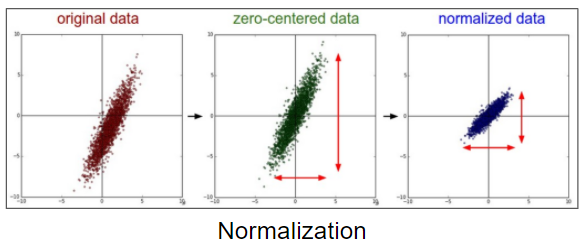
[Normalization]
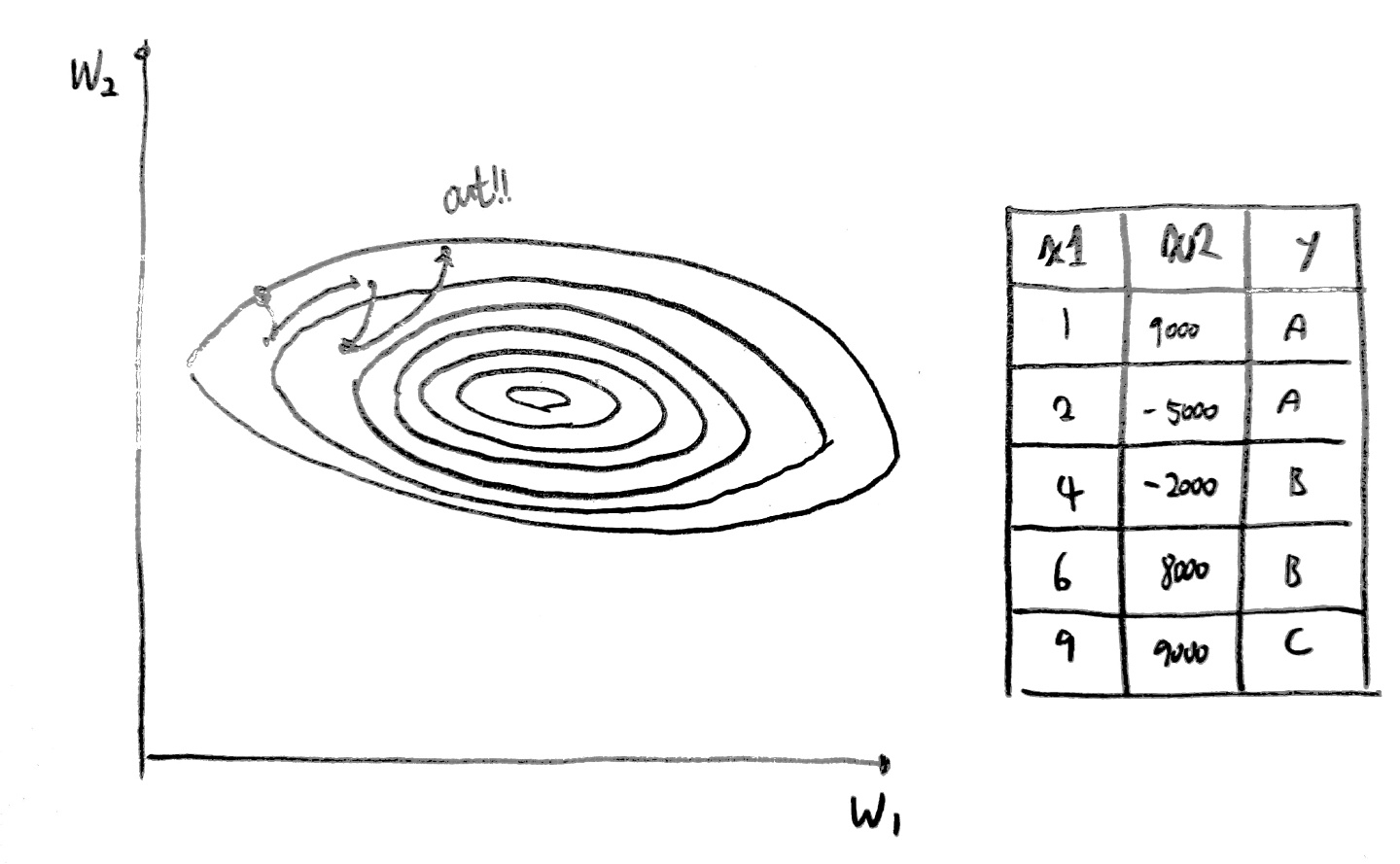
다음과 같이 x1, x2의 크기가 서로 너무 큰 차이를 보일 경우 w1, w2의 값의 차이 역시 커지며
cost값을 최적화할 때 오히려 작은 값으로 수렴하는 것이 아닌, 그래프의 바깥으로 나가게 되는 현상이 발생한다.
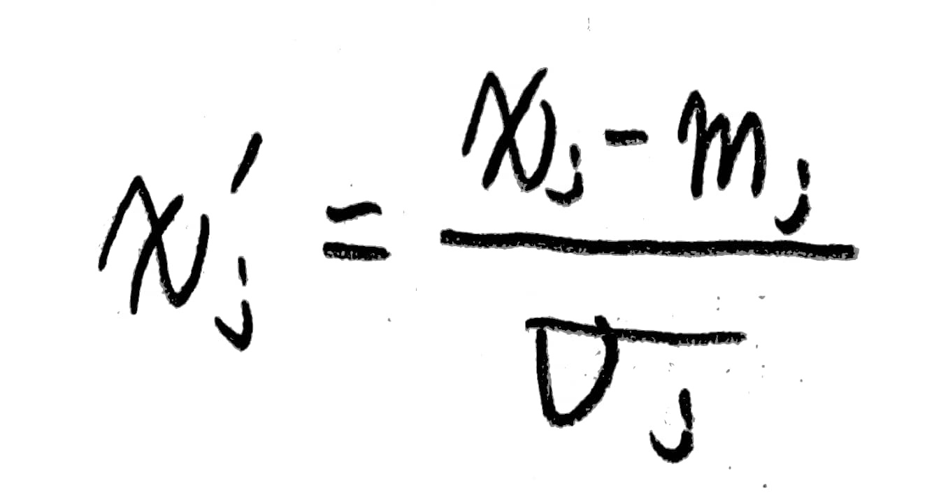
이를 해결하기 위해 normalization을 수행해야한다.
보통 선처리라 불리는 이 작업은 일정한 범위안에 데이터가 들어갈 수 있도록 크기를 변경하는 것을 의미한다.
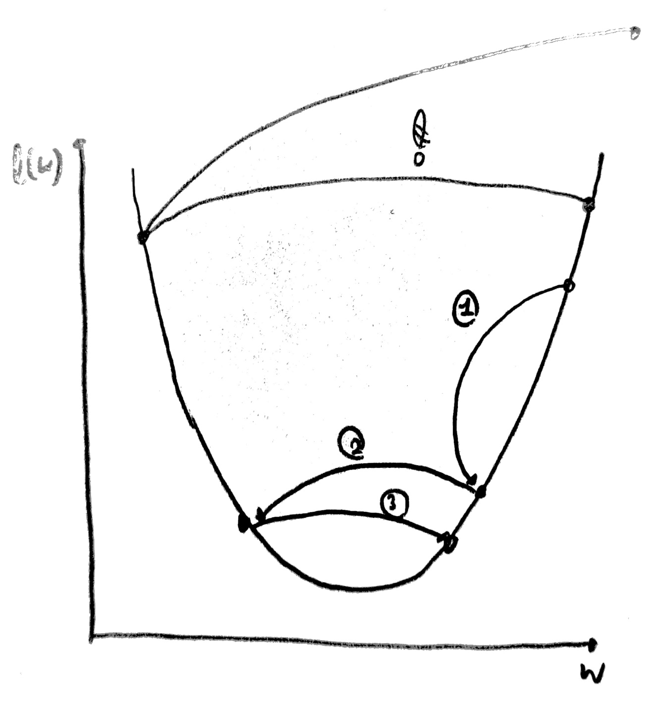
[Overfitting]
데이터의 수가 너무 적어 모든 상황에 대해 예측할 수 없는 모델이 만들어질 수 있다.
즉, 특수한 상황에 맞춰진 모델이 생성될 수 있다는 것이다.
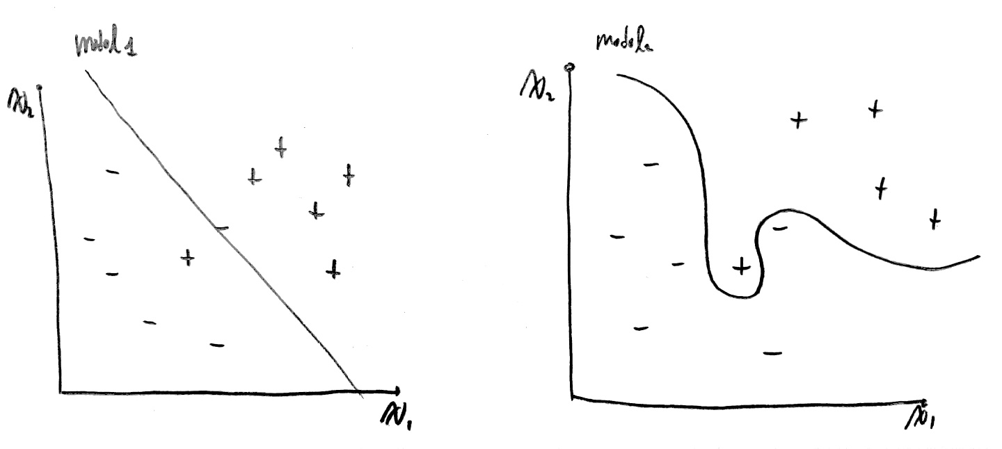
위 그래프에서 model1의 경우 많은 학습 데이터를 가지고 만든 모델에 대한 결과이다.
model1의 경우 몇몇 특수한 상황으로 인해 값이 비정상적으로 치우친 +, -에 대해선 올바르지 않은 판단을 내리겠지만, 일반적인 상황에서 올바른 판단을 내리는 모델이 된다.
만약 학습 데이터에서 비정상적으로 치우쳐진 잘못된 데이터가 있다면,
이러한 데이터를 개발자가 잘 수정하여 올바른 모델을 만들 수 있도록 해야할 것이다.
또한 특수한 상황에서도 올바른 결과를 도출할 수 있는 인공지능도 존재한다.
하지만, model2의 경우 적은 수의 데이터를 가지고 학습을 했기 때문에 특수한 상황에서의 값만을 예측할 수 밖에 없다.
즉, 일반적인 상황에서의 예측은 힘들다는 의미이다.
이를 해결하기 위한 방안은 3가지 존재한다.
1. training data를 많이 준비한다.
2. feature의 개수를 줄인다.
3. 정규화한다.
이때 정규화에 집중하여 생각해보자,
위 그래프에서 model2와 같이 잘못된 모습의 모델이 생성되는 이유는
정규화 없이 단순히 cost가 작아지게끔 유도하면 오히려 특정 가중치 값들이 커지면서 결과가 나빠지게 되기 때문이다.
이를 정규화시키기 위해 다음과 같은 식을 적용하여 해결한다.
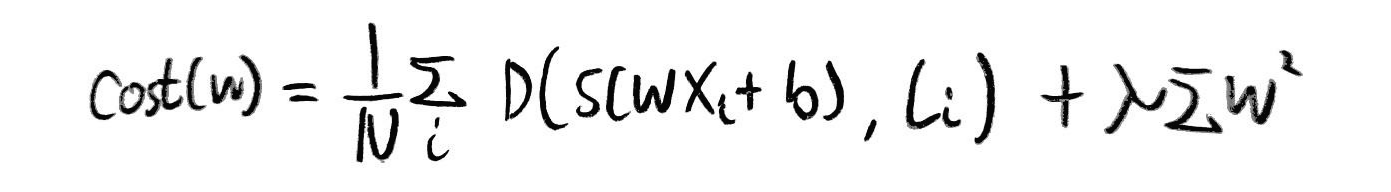
이때 cost값을 최적화할 때 람다값에 따라 regularization을 얼마나 생각해야하는가를 중점적으로 보자.
| 람다값 | 의미 |
| 1 | regularization을 중요하게 고려해야함 |
| 0 | regularization을 고려하지 않음 |
| 0.001 | regularization을 람다값만큼 고려해야함 |
[Training set, Testing set]
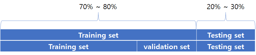
보통 30퍼센트 정도는 testing set, 나머지 70%는 training set으로 사용한다.
단, 70%에 해당하는 데이터를 한번 더 나누어 training set과 validation set으로 나누기도 한다.
validation set은 learning rate와 regularization strength의 올바른 값을 찾기 위해 사용된다.
보통 학습 후에 95% ~ 99%의 정확도가 나오면 좋은 모델이라 판단한다.
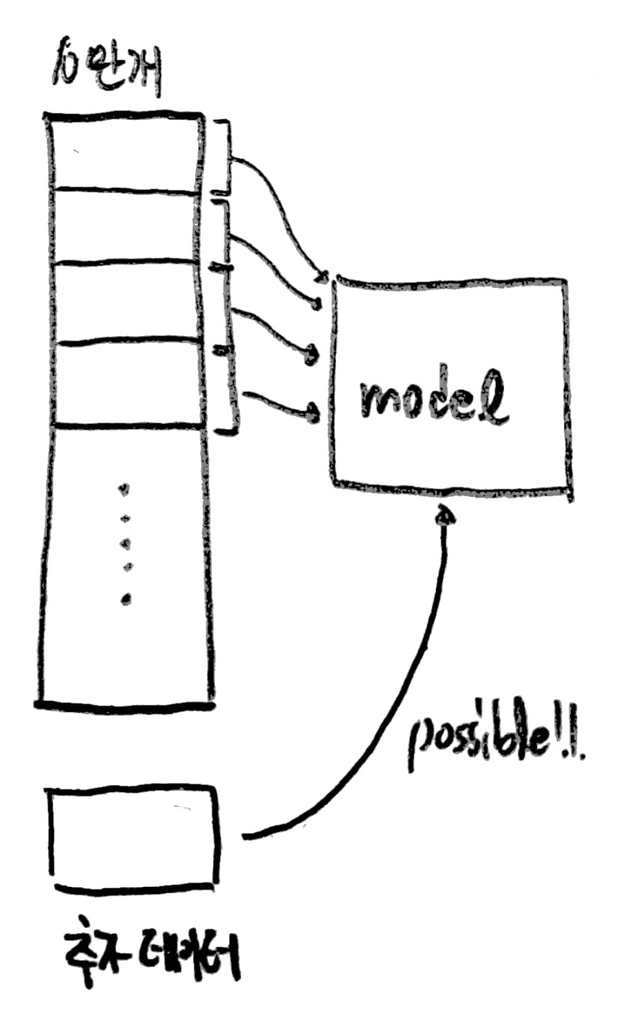
[Online Learning]
만약 10만개의 데이터를 학습시킨 후 모델을 사용하다가 추가 데이터가 도착했다고 가정해보자.
그럼 10만개의 데이터와 추가 데이터를 한꺼번에 다시 학습시켜야 할까?
이는 매우 비효율적인 일이므로 이미 학습시킨 데이터는 학습시킬 필요없이
추가로 제공받은 데이터만 기존 모델에 학습시키는 방법이 바로 online learning이다.
import tensorflow.compat.v1 as tf
tf.disable_v2_behavior()

#divide Training data and Testing data
x_data = [[1, 2, 1],
          [1, 3, 2],
          [1, 3, 4],
          [1, 5, 5],
          [1, 7, 5],
          [1, 2, 5],
          [1, 6, 6],
          [1, 7, 7]]
y_data = [[0, 0, 1],
          [0, 0, 1],
          [0, 0, 1],
          [0, 1, 0],
          [0, 1, 0],
          [0, 1, 0],
          [1, 0, 0],
          [1, 0, 0]]

x_test = [[2, 1, 1],
          [3, 1, 2],
          [3, 3, 4]]
y_test = [[0, 0, 1],
          [0, 0, 1],
          [0, 0, 1]]

X = tf.placeholder("float", [None, 3])
Y = tf.placeholder("float", [None, 3])
W = tf.Variable(tf.random_normal([3, 3]))
b = tf.Variable(tf.random_normal([3]))

hypothesis = tf.nn.softmax(tf.matmul(X, W) + b)
cost = tf.reduce_mean(-tf.reduce_sum(Y*tf.log(hypothesis), axis=1))
optimizer = tf.train.GradientDescentOptimizer(learning_rate=0.1).minimize(cost)
# Big learning rate make problems
# optimizer = tf.train.GradientDescentOptimizer(learning_rate=1.5).minimize(cost)
# Small learning rate make problems
# optimizer = tf.train.GradientDescentOptimizer(learning_rate=1e-10).minimize(cost)
prediction = tf.arg_max(hypothesis, 1)
is_correct = tf.equal(prediction, tf.arg_max(Y, 1))
accuracy = tf.reduce_mean(tf.cast(is_correct, tf.float32))

with tf.Session() as sess:
    sess.run(tf.global_variables_initializer())
    for step in range(201):
        cost_val, W_val, _ = sess.run([cost, W, optimizer], feed_dict={X: x_data, Y: y_data})
        print(step, cost_val, W_val)
    print("Prediction:", sess.run(prediction, feed_dict={X: x_test}))
    print("Accuracy:", sess.run(accuracy, feed_dict={X: x_test, Y: y_test}))
import tensorflow.compat.v1 as tf
tf.disable_v2_behavior()
import numpy as np

def min_max_scaler(data):
    numerator = data - np.min(data, 0)
    denominator = np.max(data, 0) - np.min(data, 0)
    # noise term prevents the zero division
    return numerator / (denominator + 1e-7)

#특별히 큰 x값이 index2에 존재하는 것을 확인할 수 있음
xy = np.array([[828.659973, 833.450012, 908100, 828.349976, 831.659973],
               [823.02002, 828.070007, 1828100, 821.655029, 828.070007],
               [819.929993, 824.400024, 1438100, 818.97998, 824.159973],
               [816, 820.958984, 1008100, 815.48999, 819.23999],
               [819.359985, 823, 1188100, 818.469971, 818.97998],
               [819, 823, 1198100, 816, 820.450012],
               [811.700012, 815.25, 1098100, 809.780029, 813.669983],
               [809.51001, 816.659973, 1398100, 804.539978, 809.559998]])

xy = min_max_scaler(xy)

x_data = xy[:, 0:-1]
y_data = xy[:, [-1]]

X = tf.placeholder(tf.float32, shape=[None, 4])
Y = tf.placeholder(tf.float32, shape=[None, 1])
W = tf.Variable(tf.random_normal([4, 1]), name='weight')
b = tf.Variable(tf.random_normal([1]), name='bias')

hypothesis = tf.matmul(X, W) + b
cost = tf.reduce_mean(tf.square(hypothesis - Y))
optimizer = tf.train.GradientDescentOptimizer(learning_rate=1e-5)
train = optimizer.minimize(cost)

sess = tf.Session()
sess.run(tf.global_variables_initializer())
for step in range(2001):
    cost_val, hy_val, _ = sess.run([cost, hypothesis, train], feed_dict={X: x_data, Y: y_data})
    print(step, "Cost:", cost_val, "\nPrediction:\n", hy_val)

#정규화된 데이터 확인해보기
print(xy)
이제부터 나올 코드는 mnist라는 dataset을 사용한 코드이다.
이때 새로운 개념인 epoch가 등장하는데 정리하자면 다음과 같다.
| 단어 | 뜻 |
| epoch | 모든 데이터를 한번 학습했을 때의 단위 |
| batch | 메모리 공간은 한계가 존재하므로 학습 데이터를 나눠 차례대로 올려 사용하는데, 이때 메모리에 올리는 학습 데이터의 총 개수 |
| iterator | 하나의 batch인 학습 데이터를 학습했을 때의 단위 |
예를 들면 다음과 같다.
"만약 1000개의 학습 데이터가 있고, batch 크기가 500일 때,
2번의 iterator를 거치면 1개의 epoch이 완료된다."
import tensorflow.compat.v1 as tf
import matplotlib.pyplot as plt
import numpy as np
import random
tf.disable_v2_behavior()

mnist = tf.keras.datasets.mnist
(x_train, y_train), (x_test, y_test) = mnist.load_data()
# 하나의 행으로 모든 이미지 데이터를 받음
# 60000개의 이미지를 로드함

print(len(x_train), len(y_train), x_train.shape, y_train.shape)
print(len(x_test), len(y_test), x_test.shape, y_test.shape)

x_train, x_test = x_train/255.0, x_test/255.0

nb_classes = 10

#사진 하나당 28*28 픽셀이므로 총 784개의 픽셀임
x_train_new = x_train.reshape(len(x_train), 784)   #60000 * 784 배열로 변경 - 한행당 이미지 하나
y_train_new = np.zeros((len(y_train), nb_classes)) #60000 * 10 배열 생성
for i in range(len(y_train_new)):
  y_train_new[i,y_train[i]] = 1                    #one-hot encoding

x_test_new = x_test.reshape(len(x_test), 784)      #60000 * 784 배열로 변경 - 한행당 이미지 하나
y_test_new = np.zeros((len(y_test), nb_classes))   #60000 * 10 배열 생성
for i in range(len(y_test_new)):
  y_test_new[i,y_test[i]] = 1                      #one-hot encoding

# image of shape 28 * 28 = 784
X = tf.placeholder(tf.float32, [None, 784])
Y = tf.placeholder(tf.float32, [None, nb_classes])   #6만개의 학습에 대한 10개의 가설 결과

W = tf.Variable(tf.random_normal([784, nb_classes])) #가설이 10개이고 가설별로 784개의 weigh을 가짐, 즉 7840개의 w
b = tf.Variable(tf.random_normal([nb_classes]))      #가설이 10개니 가설의 b도 10

# 다중 분류이므로 softmax사용
hypothesis = tf.nn.softmax(tf.matmul(X, W) + b)

#cross entropy
cost = tf.reduce_mean(-tf.reduce_sum(Y * tf.log(hypothesis), axis=1))
optimizer = tf.train.GradientDescentOptimizer(learning_rate=0.1).minimize(cost)

is_correct = tf.equal(tf.arg_max(hypothesis, 1), tf.arg_max(Y, 1))
accuracy = tf.reduce_mean(tf.cast(is_correct, tf.float32))

# parameters
training_epochs = 15
batch_size = 100
total_batch = int(len(x_train_new) / batch_size)

with tf.Session() as sess:
    sess.run(tf.global_variables_initializer())
    for epoch in range(training_epochs):
        avg_cost = 0

        for i in range(total_batch):
            batch_xs = x_train_new[(epoch * batch_size):(epoch + 1) * batch_size]
            batch_ys = y_train_new[(epoch * batch_size):(epoch + 1) * batch_size]

            _, cost_val = sess.run([optimizer, cost], feed_dict={X: batch_xs, Y: batch_ys})
            avg_cost += cost_val / total_batch

        print("Epoch: {:04d}, Cost: {:.9f}".format(epoch + 1, avg_cost))

    print("Accuracy: ", accuracy.eval(session=sess, feed_dict={X: x_test_new, Y: y_test_new}))

    random_idx = random.randrange(1,10000)
    print ("random_idx : ", random_idx)
    print("Prediction: ", sess.run(tf.argmax(hypothesis, 1), feed_dict={X: x_test_new[random_idx : random_idx + 1]}))

    plt.imshow(
        x_test_new[random_idx : random_idx + 1].reshape(28, 28),
        cmap="Greys",
        interpolation="nearest",
    )
plt.show()'AI > 모두를 위한 딥러닝 정리' 카테고리의 다른 글
| Day9. Neural Network and TensorBoard code (0) | 2022.04.19 |
|---|---|
| Day8. Basic information for Neural Network (0) | 2022.04.18 |
| Day6. Softmax (0) | 2022.04.11 |
| Day5. Logistic Classification과 Logistic Regression (0) | 2022.04.01 |
| Day4. multi-variable linear regression (0) | 2022.03.21 |


댓글